Spherical linear interpolation in WebAssembly 3.0

Summary

In this article, a branch-free implementation of SLERP is presented for Web graphics, targeting the WebAssembly 3.0 [1] standard. The presented formulation does not depend on trigonometric functions from a standard library or the computing platform, which is particularly appealing for small code size overhead on the web. The final code fits in 417 bytes of branch-free WebAssembly code.

Emphasis is placed on a presentation of step by step optimizations that lead up to the final code, rather than provide it as if by magic.

Introduction

Given two unit direction vectors, or unit quaternions `from` and `to`, and an interpolation time parameter `t: [0, 1]`, the task is to smoothly interpolate `from → to` as `t` ranges `0 → 1`.

function NLERP_dir(vec from, vec to, float t) {
  return normalize(from*(1-t) + to*t);
}

A straightforward way to achieve this for normalized direction vectors is to linearly interpolate and then re-normalize, or NLERP (Listing 1).

This algorithm will produce a continuous motion, but as a drawback, the angular velocity of the animation will fluctuate. The reason for this is depicted interactively in Figure 1, which shows a worst case scenario for NLERP in red when the input vectors `from` and `to` are pointing in the opposite directions.

This article focuses on the interpolation of 3D rotation frames using quaternions [2]. The discussion that follows assumes that the reader is already familiar with quaternion mathematics. For a refresher, the Technical Report "Quaternions, Interpolation and Animation" [3] by Dam, Koch and Lillholm from the University of Copenhagen is recommended for the mathematically oriented readers. For readers coming from a software engineering background, the presentation "Understanding Quaternions" [4] by Jim Van Verth from GDC 2013 provides a more hands-on context.

The `NLERP_dir` example from Listing 1 can be adapted from 3D vector case to 4D quaternion mathematics with only a small change, shown in pseudo-code in Listing 2.

function NLERP(quat from, quat to, float t) {
  if (from·to < 0) from = -from;
  return normalize(from*(1-t) + to*t);
}

Because each 3D rotation frame has two equivalent representations as quaternions, i.e. `q` and `-q` encode the same orientation, it is important to ensure that the interpolation takes place over the shortest arc by negating one of the inputs if the 4D dot product is negative. NLERPing two quaternions residing on the opposite hemispheres of the 4D unit hypersphere would result in animated interpolation about the same axis, but winding the long way around via the opposite rotation direction as the time parameter `t` traces from `0` to `1`.

Some authors establish interpolating via the long arc to be a feature ([5]) or that data should be preprocessed to avoid that from happening ([6]), but for the purposes of convention and promoting general purpose code, it is simpler to take the short arc rotation as the standard to avoid confusion. This is the approach taken for example by the GLTF model interchange specification ([7]).

Throughout this article, all presented code will contain the 4D hemisphere dot product check to perform short-arc rotations only.

To fix NLERP to interpolate with constant angular velocity, it turns out that only a small tweak to the interpolation weights is necessary.

This tweak was published by Ken Shoemake in "Animating Rotation with Quaternion Curves" [8] in SIGGRAPH'85, attributed to Glenn Davis. The SLERP algorithm is:

function SLERP(quat from, quat to, float t) {
  if (from·to < 0) from = -from;
  Ω = cos⁻¹(from·to);
  return sin((1-t)Ω)/sinΩ*from + sin(tΩ)/sinΩ*to;
}

In Figure 1, the SLERP algorithm is depicted in blue, illustrating how the biasing of interpolation weights results in rotating direction vectors with constant angular velocity.

The reason why these rebiased interpolation weights produce the sought constant angular velocity rotation is beyond the scope of this article. The interested reader can consult a short geometric proof in Chapter 4.6.3 of Mathematics for 3D Game Programming and Computer Graphics, Third Edition by Eric Lengyel ([9]).

Figure 2 takes the direction vector rotation example from Figure 1 to 3D rotation frames, and visualizes rotating a 3D cube using both SLERP and NLERP using keyframed animation with consecutive keyframes of 180 degree rotations. Rotation using SLERP has steady constant angular velocity, whereas angular velocity with NLERP has an oscillating behavior.

When interpolating 3D rotation frames, the maximum angle error between NLERP and SLERP is at most 8.1491° (see Figure 21 later in this article), enough to cause a visually observable discrepancy in both position and angular velocity.

Why WebAssembly?

The internet and GitHub contain decades' worth of implementations of the SLERP function in different languages, and targeting different hardware SIMD instruction sets and standard libraries. But WebAssembly does not natively support SSE or NEON. This means that a SLERP function that is tuned for a specific precision/performance trade-off balance for native CPUs, may not perform as expected if ported over as-is to WebAssembly.

In particular, there are a couple of differences that motivate writing new code for SLERP for WebAssembly:

• WebAssembly provides SIMD capabilities using a virtual SIMD instruction set architecture (<wasm_simd128.h> [10] in LLVM/Clang) and does not provide direct SSE/NEON instruction API. While Emscripten does support compilation of SSE/NEON intrinsics utilizing C code [11] (the author contributed SSE/AVX compilation capabilities to Emscripten), that SSE/NEON emulation causes overhead for vector intrinsics that do not have a 1:1 mapping to the WebAssembly virtual SIMD instruction set.
• On native platforms, the error metrics of a SLERP implementation may be tuned for the use of the SIMD approximate reciprocal square root `rsqrt()` instruction, which is not available in WebAssembly SIMD.
• On Intel x86, SSE computation has the capability to seamlessly alias a CPU register between SIMD scalar (`*ss`) and packed (`*ps`) calculations, which WebAssembly SIMD does not have.
• On native platforms, calling standard C math library `sinf()` and `acosf()` functions may be more performant or be inlined and SIMD-vectorized by the compiler. With Emscripten, these trigonometric functions either use the Musl libc library, or call out across the WebAssembly→JavaScript virtual machine boundary to JavaScript's double-precision `Math.sin()` trigonometric functions. Both implementations are tuned (for obvious reasons) for high precision rather than real-time games/graphics precision-performance trade-off.
• On native platforms, the compiled code size on disk is immaterial, whereas on the web, compiled code size is everything since all code needs to be downloaded on first site visit while the user expects an immediate site load experience.

The WebAssembly Relaxed SIMD extension was ratified to Phase 4 in March 2023 [12] and both modern browsers Firefox and Chrome have supported it ([13]) since 2023. The WebAssembly 3.0 standard was released in September 2025 and includes the Relaxed SIMD instruction set. The Relaxed SIMD API is interesting in this context since it adds vectorized Fused Multiply-Add (FMA) [14] capability to WebAssembly.

With the above computing platform differences in mind, let's take a look at designing a new formulation for SLERP, which performs well when targeting WebAssembly 3.0 with the Emscripten compiler.

Baseline implementation

To get going, we will need a baseline implementation to compare correctness and performance against. For that purpose, let's implement a "ground truth" version in JavaScript's double-precision floating point.

function slerpReference(from, to, t) {
  let x0 = from.x;
  let y0 = from.y;
  let z0 = from.z;
  let w0 = from.w;

  let x1 = to.x;
  let y1 = to.y;
  let z1 = to.z;
  let w1 = to.w;

  let cosOmega = x0*x1 + y0*y1 + z0*z1 + w0*w1;

  if (cosOmega < 0) {
    x0 = -x0;
    y0 = -y0;
    z0 = -z0;
    w0 = -w0;
    cosOmega = -cosOmega;
  }

  // Avoid division by sinOmega≈0 when the quaternions are nearly identical,
  // but also avoid accidentally calling Math.acos(1.00001) or so.
  if (cosOmega >= 0.999) {
    return {
      x: (1 - t)*x0 + t*x1,
      y: (1 - t)*y0 + t*y1,
      z: (1 - t)*z0 + t*z1,
      w: (1 - t)*w0 + t*w1
    };
  }

  const omega = Math.acos(cosOmega);
  const sinOmega = Math.sin(omega);

  const a = Math.sin((1 - t) * omega) / sinOmega;
  const b = Math.sin(t * omega) / sinOmega;

  return {
    x: a*x0 + b*x1,
    y: a*y0 + b*y1,
    z: a*z0 + b*z1,
    w: a*w0 + b*w1
  };
}

The implementation in Listing 4 takes the SLERP pseudo-code otherwise literally, but has an added check for `if (cosOmega >= 0.999)`. That could cause both lerp weights `(1 - t) * omega` and `t * omega` to vanish to zero, and at `cosOmega=1`, `sinOmega` would also divide by zero. Also due to numerical imprecision, `cosOmega` might actually have a value slightly above one, in which case `Math.acos(1.00001)` would return `NaN`.

The situation `cosOmega >= 0.999` occurs if the two input quaternions `from` and `to` nearly coincide, so in that case, one could return either `from` or `to` as-is since they are virtually the same, but this reference implementation will revert to interpolating by `t` between the two (for a reason that becomes apparent later).

Mathematically the above implementation is solid, but there is however a practical software engineering problem. Under animation, the slerp function may be getting iterated over multiple frames, so that the output of a previous slerp is reused as a start/endpoint to a subsequent slerp. In the above code, there is no guard against floating-point normalization drift so over time the length of interpolated quaternions may diverge from one. To ensure that this does not happen, we are inclined to add a renormalization step at the end for floating point stability. (Listing 5)

function normalize(q) {
  const invLen = 1 / Math.hypot(q.x, q.y, q.z, q.w);
  return {
    x: q.x * invLen,
    y: q.y * invLen,
    z: q.z * invLen,
    w: q.w * invLen
  };
}

function slerpReferenceNormalized(from, to, t) {
  return normalize(slerpReference(from, to, t));
}

This function `slerpReferenceNormalized()` will act as the ground truth version to compare against.

The reference code is the exact code that many 3D game engines and math libraries ship as-is (Unity 2022 [15], Unreal Engine 4 [16], three.js [17], GLM [18]). Due to the performance concern of this calculation, a game engine might then ship the NLERP function as a separate API, paired with a caution against SLERP performance. ([19])

It should be noted that there are several optimizations that can be employed to this JavaScript version, but since the motivation in this article is to compute in WebAssembly, the attention will shift to working on an implementation in the C programming language. Appendix C contains the final optimized version as JavaScript code.

The subsequent chapters focus on optimizing this reference code, by carefully highlighting the optimization process that gives way to the improved versions. The motivation is to enable software engineers internalize the meaning behind the final code, so they can adapt it for their own use.

The C version

The reference implementation in Listings 4 and 5 computes in 64-bit double precision floating point. In C, using single precision floating point is preferable, since the intended purpose is real-time graphics. Listing 6 presents a first reference C implementation `slerp1()`.

#include <math.h>

typedef struct {
  float x, y, z, w;
} quat;

quat normalize(quat q)
{
  float invLen = 1.f / sqrtf(q.x*q.x + q.y*q.y + q.z*q.z + q.w*q.w);
  return (quat){ q.x*invLen, q.y*invLen, q.z*invLen, q.w*invLen };
}

quat slerp1(quat from, quat to, float t)
{
  float x0 = from.x;
  float y0 = from.y;
  float z0 = from.z;
  float w0 = from.w;

  float x1 = to.x;
  float y1 = to.y;
  float z1 = to.z;
  float w1 = to.w;

  float cosOmega = x0*x1 + y0*y1 + z0*z1 + w0*w1;

  if (cosOmega < 0) {
    x0 = -x0;
    y0 = -y0;
    z0 = -z0;
    w0 = -w0;
    cosOmega = -cosOmega;
  }

  // Avoid division by sinOmega≈0 when the quaternions are nearly identical,
  // but also avoid accidentally calling acosf(1.00001f) or so.
  if (cosOmega >= 0.999f) {
    quat result = {
      (1 - t)*x0 + t*x1,
      (1 - t)*y0 + t*y1,
      (1 - t)*z0 + t*z1,
      (1 - t)*w0 + t*w1
    };
    return normalize(result);
  }

  float omega = acosf(cosOmega);
  float sinOmega = sinf(omega);

  float a = sinf((1 - t) * omega) / sinOmega;
  float b = sinf(t * omega) / sinOmega;

  quat result = {
    a*x0 + b*x1,
    a*y0 + b*y1,
    a*z0 + b*z1,
    a*w0 + b*w1
  };

  return normalize(result);
}

The C code in Listing 6 is a faithful translation of the JavaScript reference slerp function from Listings 4 and 5 to C. 1. SLERP time, ns/call (C/Wasm vs JS)

Click the button to start measuring. Each animation frame runs 100k random slerps in C (Wasm), verifies each against the JS reference, and adds a new sample to the graphs below.

Click the button to start measuring. Each animation frame runs 100k random slerps in C (Wasm), verifies each against the JS reference, and adds a new sample to the graphs below.

Click the button to start measuring. Each animation frame runs 100k random slerps in C (Wasm), verifies each against the JS reference, and adds a new sample to the graphs below.

Classic optimizations

To begin improving on `slerp1()`, let's apply some common optimizations.

First, observe that since we have decided to `normalize()` the output vector, it means that we can remove the trigonometric `sin(omega)` call and the division from the denominator altogether. Normalization is certainly cheaper than evaluating a transcendental function. (Listing 7)

quat slerp2(quat from, quat to, float t)
{
  float x0 = from.x;
  float y0 = from.y;
  float z0 = from.z;
  float w0 = from.w;

  float x1 = to.x;
  float y1 = to.y;
  float z1 = to.z;
  float w1 = to.w;

  float cosOmega = x0*x1 + y0*y1 + z0*z1 + w0*w1;

  if (cosOmega < 0) {
    x0 = -x0;
    y0 = -y0;
    z0 = -z0;
    w0 = -w0;
    cosOmega = -cosOmega;
  }

  // Avoid multiplication by very small omega from crushing precision in sinf()
  // when the input quaternions are nearly identical.
  if (cosOmega >= 0.999f) {
    quat result = {
      (1 - t)*x0 + t*x1,
      (1 - t)*y0 + t*y1,
      (1 - t)*z0 + t*z1,
      (1 - t)*w0 + t*w1
    };
    return normalize(result);
  }

  float omega = acosf(cosOmega);

  float a = sinf((1 - t) * omega);
  float b = sinf(t * omega);

  quat result = {
    a*x0 + b*x1,
    a*y0 + b*y1,
    a*z0 + b*z1,
    a*w0 + b*w1
  };

  return normalize(result);
}

Then, let's apply a small structural cleanup to unify the control flow of both `return` paths in the code. (Listing 8)

quat slerp3(quat from, quat to, float t)
{
  float x0 = from.x;
  float y0 = from.y;
  float z0 = from.z;
  float w0 = from.w;

  float x1 = to.x;
  float y1 = to.y;
  float z1 = to.z;
  float w1 = to.w;

  float cosOmega = x0*x1 + y0*y1 + z0*z1 + w0*w1;

  if (cosOmega < 0) {
    x0 = -x0;
    y0 = -y0;
    z0 = -z0;
    w0 = -w0;
    cosOmega = -cosOmega;
  }

  float a = 1 - t;
  float b = t;

  // Avoid multiplication by very small omega from crushing precision in sinf()
  // when the input quaternions are nearly identical.
  if (cosOmega < 0.999f) {
    float omega = acosf(cosOmega);
    a = sinf(a * omega);
    b = sinf(b * omega);
  }

  quat result = {
    a*x0 + b*x1,
    a*y0 + b*y1,
    a*z0 + b*z1,
    a*w0 + b*w1
  };

  return normalize(result);
}

The `slerp3()` function in Listing 8 shows again how the structure of the SLERP algorithm is effectively a NLERP, just with adjusted lerp weights to balance out the rotation speed. The variables `a` and `b` start off as the NLERP weights, and if the configuration is not degenerate, the lerp weights are adjusted to the SLERP reweighted factors with a bit of trigonometry.

As the next optimization, let's convert the function to utilize WebAssembly's SIMD instruction set. As for the SIMD data type, let's use the LLVM/Clang `__f32x4` Wasm SIMD vector type directly. When fitting the code into an existing engine, the data type abstractions will usually be something specific to the codebase, but for a general purpose example, it is better to keep abstraction code out of the way to focus on the topic.

The vector type `__f32x4` should be read as "`float` four times" in a single CPU SIMD register, so it is a 128-bit structure.

For developers new to SIMD programming, publicly available university course articles like Practical SIMD Programming by Jacco Bikker from Universiteit Utrecht [20] or SIMD Programming by Moreno Marzolla from Università di Bologna [21] are great ways to get up to speed quickly.

Listing 9 presents a straightforward conversion of `slerp3()` to the WebAssembly SIMD API.

// Calculates dot product a·b into all lanes of the returned vector.
static __f32x4 dp(__f32x4 a, __f32x4 b)
{
  a = wasm_f32x4_mul(a, b);
  a = wasm_f32x4_add(a, wasm_i32x4_shuffle(a, a, 1,0,3,2));
  return wasm_f32x4_add(a, wasm_i32x4_shuffle(a, a, 2,3,0,1));
}

__f32x4 slerp4(__f32x4 from, __f32x4 to, float t)
{
  __f32x4 cosOmega = dp(from, to);

  if (wasm_f32x4_extract_lane(cosOmega, 0) < 0) {
    from = wasm_f32x4_neg(from);
    cosOmega = wasm_f32x4_neg(cosOmega);
  }

  float a = 1 - t;
  float b = t;

  // Avoid multiplication by very small omega from crushing precision in sinf()
  // when the input quaternions are nearly identical.
  if (wasm_f32x4_extract_lane(cosOmega, 0) < 0.999f) {
    float omega = acosf(wasm_f32x4_extract_lane(cosOmega, 0));
    a = sinf(a * omega);
    b = sinf(b * omega);
  }

  __f32x4 v = wasm_f32x4_mul(wasm_f32x4_splat(a), from);
  __f32x4 w = wasm_f32x4_mul(wasm_f32x4_splat(b), to);
  __f32x4 ret = wasm_f32x4_add(v, w);

  __f32x4 len = wasm_f32x4_sqrt(dp(ret, ret));
  return wasm_f32x4_div(ret, len);
}

The function `slerp4()` looks more compact with the vectorized arithmetic. The earlier scalar operations on the four components of the quaternion separately are replaced by vector intrinsic instructions in WebAssembly SIMD.

As the next change, let's work towards making the function branchless by easing the first `if()` branch. This is not the most critical performance thing (the transcendentals are the real problem), but let's apply the following small improvements first.

1. The vectorized scalar `cosOmega` is being negated if it is `< 0`, which is another way of saying to take the absolute value. WebAssembly SIMD has a dedicated intrinsic `wasm_f32x4_abs()` for that. Note that this is a virtual instruction - the SSE instruction set does not have a native float absolute value instruction. The WebAssembly VM will attempt to find the best set of SSE instructions to take an absolute value, letting us enjoy a small byte size encoding of this operation on disk.
2. If `cosOmega < 0`, the first branch ensures we are calculating `v = a*(-from)`. But that is the same as calculating `v = (-a)*from`. So let's negate `a` when `cosOmega < 0` instead of negating `from`. This seems like a frivolous change at this point, but it manifests into a concrete optimization later.

Putting these two changes together gives Listing 10.

__f32x4 slerp5(__f32x4 from, __f32x4 to, float t)
{
  __f32x4 cosOmega = dp(from, to);

  float a = 1 - t;
  float b = t;

  if (wasm_f32x4_extract_lane(cosOmega, 0) < 0) {
    a = -a;
  }
  cosOmega = wasm_f32x4_abs(cosOmega);

  // Avoid multiplication by very small omega from crushing precision in sinf()
  // when the input quaternions are nearly identical.
  if (wasm_f32x4_extract_lane(cosOmega, 0) < 0.999f) {
    float omega = acosf(wasm_f32x4_extract_lane(cosOmega, 0));
    a = sinf(a * omega);
    b = sinf(b * omega);
  }

  __f32x4 v = wasm_f32x4_mul(wasm_f32x4_splat(a), from);
  __f32x4 w = wasm_f32x4_mul(wasm_f32x4_splat(b), to);
  __f32x4 ret = wasm_f32x4_add(v, w);

  __f32x4 len = wasm_f32x4_sqrt(dp(ret, ret));
  return wasm_f32x4_div(ret, len);
}

The optimizations added for the `slerp5()` version did not completely eliminate the first `if()` branch, but we are almost there.

Approximating sin()

The performance of the `slerp5()` function is dominated by the trigonometric `sinf()` and `acosf()` calls. For real-time graphics, all that precision that the standard library trig functions provide is not really needed, so let's replace `sinf()` by a quick-to-evaluate fifth order polynomial approximation.

As a simple implementation, one could use e.g. the Maclaurin series [22] approximation cut off to the first terms for performance (Figure 3),

sin(x) ≈ x - x³/6 + x⁵/120

but the error generated by this polynomial is rather high as `|x|` grows away from zero. A better approximation is found by applying Chebyshev's equioscillation theorem [23] across `x ∈ [-π/2, π/2]` using Python's numpy and mpmath packages (Appendix G), which yields the polynomial in Figure 4.

sin(x) ≈ 0.9996967731390435*x - 0.16567307932054615*x³ + 0.007514377178300066*x⁵

Throughout the rest of the article, these kinds of numerical coefficients will be present. Even though single-precision floating point computation will be used in C, these constants have been calculated and are presented to be accurate up to the double-precision floating point limit. The purpose here is that since program code is often copy-pasted and adapted to different languages, retaining 64 bits of precision with magic constants enables avoiding precision loss when going from a float32 context to a float64 context.

How good is the approximation in Figure 4 compared to the Maclaurin polynomial? Let's plot both approximations against the actual `sin(x)` in the range `x ∈ [-π/2, π/2]`, which is the range where slerp needs to evaluate the sine function. (Figure 5)

The graphs are visually the same so the approximation should not be obviously bad at least. Let's instead plot the maximum absolute error to understand better (Figure 6).

The Maclaurin polynomial's error reaches ~0.00452 at `x=±π/2`, whereas the Chebyshev polynomial's maximum error over the range is only ~0.0000677 (at the equioscillation points, like `x=-1.4139...`). The Chebyshev polynomial is a better fit.

So by using the function in Listing 11 instead of calling to `sinf()`, we are introducing only a 6.77e-5 error over the true sine function at `x ∈ [-π/2, π/2]`.

static float approx_sin(float x)
{
  float xx = x*x;
  return x * (xx * (0.007514377178300066f * xx - 0.16567307932054615f) + 0.9996967731390435f);
}

The function `approx_sin` is very quick to calculate, coming out at only 4 MULs and 2 ADDs.

In fact, let's immediately go a step further. Rather than calculating just one `approx_sin()` at a time, we can immediately SIMDify the function to calculate four sines in one go. We will only really need two, but SIMD vectors are 4-wide at minimum. Listing 12 shows what that will look like in WebAssembly SIMD code.

#include <wasm_simd128.h>

static __f32x4 approx_sin4(__f32x4 x)
{
  __f32x4 xx = wasm_f32x4_mul(x, x);
  __f32x4 y = wasm_f32x4_relaxed_madd(wasm_f32x4_splat(0.007514377178300066f), xx, wasm_f32x4_splat(-0.16567307932054615f));
  return wasm_f32x4_mul(x, wasm_f32x4_relaxed_madd(xx, y, wasm_f32x4_splat(0.9996967731390435f)));
}

This is the first spot where Fused Multiply-Add (FMA) supported from the WebAssembly Relaxed SIMD extension can be applied. A FMA instruction calculates the function `FMA(a,b,c) := a*b+c` in a single CPU instruction. The good old Intel Intrinsics Guide [24] states for all the recent Intel μarchs (Skylake - Alder Lake) that each of vector MUL, ADD, and FMA instructions have the same latency of 4 cycles and a throughput of 0.5/cycle, so FMA is effectively a MUL and an ADD done in one go.

When evaluating polynomials that are expressed in Horner form [25] (into which the polynomials in Listings 11 and 12 are structured), all additions can be fused into the multiplication instructions for no cost.

FMA instructions save the intermediate result of the multiplication internally with better precision before addition, so they also have slightly better numerical accuracy. Technically this means that the error analysis presented later is then sensitive to whether FMA was used or not. In WebAssembly, the "relaxed" part in Relaxed FMA means that the VM implementation can choose to fall back to a nonfused computation for example if the current CPU is so outdated as to not support true FMA instructions.

Coming back to the main body of the `slerp5` function in Listing 10, let's merge the weights `a` and `b` into a common SIMD vector so that this new `approx_sin4()` can be applied to both in one go. The result is a small change but an important one, shown in Listing 13.

__f32x4 slerp6(__f32x4 from, __f32x4 to, float t)
{
  __f32x4 cosOmega = dp(from, to);

  __f32x4 w = wasm_f32x4_make(1-t, t, 0, 0);

  if (wasm_f32x4_extract_lane(cosOmega, 0) < 0) {
    w = wasm_f32x4_replace_lane(w, 0, t-1);
  }
  cosOmega = wasm_f32x4_abs(cosOmega);

  // Avoid multiplication by very small omega from crushing precision in sinf()
  // when the input quaternions are nearly identical.
  if (wasm_f32x4_extract_lane(cosOmega, 0) < 0.999f) {
    float omega = acosf(wasm_f32x4_extract_lane(cosOmega, 0));
    w = approx_sin4(wasm_f32x4_mul(w, wasm_f32x4_splat(omega)));
  }

  __f32x4 V = wasm_f32x4_mul(wasm_i32x4_shuffle(w,w,0,0,0,0), from);
  __f32x4 W = wasm_f32x4_mul(wasm_i32x4_shuffle(w,w,1,1,1,1), to);
  __f32x4 ret = wasm_f32x4_add(V, W);

  __f32x4 len = wasm_f32x4_sqrt(dp(ret, ret));
  return wasm_f32x4_div(ret, len);
}

In function `slerp6()`, both of the trigonometric `sin()` calls were replaced with the new approximation, but after packing `a` and `b` into a SIMD vector, the first `if (wasm_f32x4_extract_lane(cosOmega, 0) < 0)` branch starts to look particularly awkward. The branch is extracting the scalar out from the SIMD register, and then putting an updated one back in. Back-and-forth scalar↔SIMD data juggling is generally not good shape for fast SIMD code.

Eyeballing that branch construct, what is happening there is that if `cosOmega < 0`, we want to flip the sign bit of `w[0]`. Since the sign bit is orthogonal to the value bits on floating-point numbers (and not like 2's complement on integers), we can achieve that sign transfer/swap calculation in branchless SIMD fashion by a small AND+XOR sequence. Listing 14 shows this transformation.

__f32x4 slerp7(__f32x4 from, __f32x4 to, float t)
{
  __f32x4 cosOmega = dp(from, to);

  __f32x4 w = wasm_f32x4_make(1-t, t, 0, 0);

  // Flip 1-t to t-1 if cosOmega < 0
  w = wasm_v128_xor(w, wasm_v128_and(cosOmega, wasm_i32x4_make(0x80000000u, 0, 0, 0)));
  cosOmega = wasm_f32x4_abs(cosOmega);

  // Avoid multiplication by very small omega from crushing precision in sinf()
  // when the input quaternions are nearly identical.
  if (wasm_f32x4_extract_lane(cosOmega, 0) < 0.999f) {
    float omega = acosf(wasm_f32x4_extract_lane(cosOmega, 0));
    w = approx_sin4(wasm_f32x4_mul(w, wasm_f32x4_splat(omega)));
  }

  __f32x4 V = wasm_f32x4_mul(wasm_i32x4_shuffle(w,w,0,0,0,0), from);
  __f32x4 W = wasm_f32x4_mul(wasm_i32x4_shuffle(w,w,1,1,1,1), to);
  __f32x4 ret = wasm_f32x4_add(V, W);

  __f32x4 len = wasm_f32x4_sqrt(dp(ret, ret));
  return wasm_f32x4_div(ret, len);
}

In function `slerp7()` the first branch is now removed altogether. It would be nice to be able to remove the remaining second branch as well. We will do that as a by-product while we approximate the `cos⁻¹()` function.

Approximating cos⁻¹()

Since the Chebyshev minimax polynomial approximation to `sin()` with just a 5th degree polynomial worked out so well, the first thought is to apply the same idea to `cos⁻¹()` as well.

Unfortunately it turns out that `cos⁻¹()` is a bit trickier to approximate with just a simple polynomial, because its derivative (`-1/sqrt(1-x²)`) has a singularity at `x = 1`. Straightforward attempts yield the functions in Figure 7.

acos3(x) ≈ x * (-0.9157956 *x*x - 0.49146938) + 1.48903066

acos5(x) ≈ x * ((-1.64231191 *x*x + 1.56149304) *x*x - 1.48997746) + 1.62368143

Computationally either of `acos3()` or `acos5()` would be pleasant since they would have a 2-3 FMAs plus one MUL structure. Let's plot these approximations against the true `cos⁻¹(x)` function (Figure 8).

Unfortunately it is evident that the precision of these approximations is nowhere near accurate to the true `cos⁻¹(x)` function like was the case with `sin(x)` in Figure 5 from the previous chapter. The problem is the singularity at `x = 1`, which is very un-polynomial-like, so approximating polynomials that are truncated off at low degrees will struggle to mimic `cos⁻¹(x)`.

However, hope is not lost. There are two interesting observations to make.

First, the `slerp()` function only ever invokes `cos⁻¹(x)` in the `x ∈ [0, 1]` range, so any error in the approximating polynomial outside that range will not matter.

Second, we care little about the precision of the approximation of `cos⁻¹(x)` as `x → 1.0`, because the closer the argument is to one, the closer the two slerp input quaternions are to each other anyway. Near `x≈1.0` input value to `cos⁻¹(x)` the two input quaternions `from` and `to` are effectively the same quaternion to begin with, so a dramatic loss in precision in our approximation can be endured. The approximating polynomial of choice can return anything frivolous, like `cos⁻¹(1) ≈ 0.5` or `cos⁻¹(1) ≈ 1` and the overall slerp error would still be zero.

That gives an idea. Because the `slerp7()` function still has that one unpleasant `if()` branch that needs to guard against `cos⁻¹(x)` returning zero when `x≈1.0`, let's choose an approximating polynomial in a way for which this zero does not happen. Then we can simply delete that `if()` branch completely, since the singularity is avoided.

That is, the true value of `cos⁻¹(1)` is zero, but we actually want our interpolating polynomial to return anything but!

In general terms, the precision of our approximation is more important when `x` is smaller, and less so when `x` is closer to one. The key insight is that we want to find an approximating polynomial that minimizes the total slerp output error, and not the error vs the `cos⁻¹(x)` function itself.

So instead of chasing after minimizing the maximum approximation error to the `cos⁻¹(x)` function, Chebyshev minimax polynomial coefficients were generated over the first half of the range and then a computer search that minimizes the total magnitude error of the `slerp()` function was undertaken. This was done by iterating with an ad hoc hill climb search loop that nudged units in the last place (ULP) [26] of `a`, `b`, `c` and `d` coefficients in a polynomial of shape `cos⁻¹(x) ≈ a + b*x + c*x² + d*x³` while measuring the overall squared difference error in the `slerp()` output against a ground truth double precision slerp.

The computer search converged to the approximating polynomial coefficients shown in Figure 9.

cos⁻¹(x) ≈ x*(x*(x*-0.627160617651148722 + 0.366191412084127366) - 1.06803417726155914) + 1.57316997572997042

The approximating function in Figure 9 is as straightforward to implement as the approximation of sine in the previous chapter. Let's write the code directly in the SIMD form so that four arguments can be evaluated at once. Listing 15 shows that only three FMA operations will be needed.

static __f32x4 crude_acos4(__f32x4 x)
{
  __f32x4 a = wasm_f32x4_relaxed_madd(x, wasm_f32x4_splat(-0.627160617651148722f),
                                         wasm_f32x4_splat(0.366191412084127366f));
  a = wasm_f32x4_relaxed_madd(a, x, wasm_f32x4_splat(-1.06803417726155914f));
  return wasm_f32x4_relaxed_madd(a, x, wasm_f32x4_splat(1.57316997572997042f));
}

What does this `crude_acos4()` approximation look like against the true `cos⁻¹(x)` function? Figure 10 plots them both and Figure 11 shows the absolute error.

Compared to the Minimax approximations in Figure 7, this crude approximation looks much cleaner.

The crude polynomial is able to hold up with `cos⁻¹(x)` up to `x ∈ [0, ~0.8]` range and then gives up attempting to follow the function to the singularity as `x → 1.0`. That is alright, as precision near `x → 1.0` does not matter as much since the input quaternions will be closer to each other then to begin with anyway.

And what is important, `crude_acos4(x) > 0` across the relevant range (`crude_acos4(1) ≈ 0.29577`) and this polynomial approximation can be evaluated even when the argument `x>1` due to floating point imprecision, so we do not need to have an `if()` check anymore to guard against `crude_acos4(1)` returning zero or `acosf(1.0001)` returning NaN, like we had to with the `float omega = acosf(cosOmega);` case.

With the SIMDified `crude_acos4(x)` function from Listing 15, we can transform the `slerp7()` function from Listing 14 into a pleasantly simplified form, shown in Listing 16.

__f32x4 slerp8(__f32x4 from, __f32x4 to, float t)
{
  __f32x4 cosOmega = dp(from, to);

  __f32x4 w = wasm_f32x4_make(1-t, t, 0, 0);

  // Flip 1-t to t-1 if cosOmega < 0
  w = wasm_v128_xor(w, wasm_v128_and(cosOmega, wasm_i32x4_make(0x80000000u, 0, 0, 0)));
  cosOmega = wasm_f32x4_abs(cosOmega);

  w = approx_sin4(wasm_f32x4_mul(w, crude_acos4(cosOmega)));

  __f32x4 V = wasm_f32x4_mul(wasm_i32x4_shuffle(w,w,0,0,0,0), from);
  __f32x4 W = wasm_f32x4_mul(wasm_i32x4_shuffle(w,w,1,1,1,1), to);
  __f32x4 ret = wasm_f32x4_add(V, W);

  __f32x4 len = wasm_f32x4_sqrt(dp(ret, ret));
  return wasm_f32x4_div(ret, len);
}

As one more tweak, let's apply a missing FMA opportunity to the calculation at the lerp stage with registers `V`, `W` and `ret`, to get the final form in Listing 17.

__f32x4 slerp9(__f32x4 from, __f32x4 to, float t)
{
  __f32x4 cosOmega = dp(from, to);

  __f32x4 w = wasm_f32x4_make(1-t, t, 0, 0);

  // Flip 1-t to t-1 if cosOmega < 0
  w = wasm_v128_xor(w, wasm_v128_and(cosOmega, wasm_i32x4_make(0x80000000u, 0, 0, 0)));
  cosOmega = wasm_f32x4_abs(cosOmega);

  w = approx_sin4(wasm_f32x4_mul(w, crude_acos4(cosOmega)));

  __f32x4 ret = wasm_f32x4_mul(from, wasm_i32x4_shuffle(w,w,0,0,0,0));
  ret = wasm_f32x4_relaxed_madd(to, wasm_i32x4_shuffle(w,w,1,1,1,1), ret);

  __f32x4 len = wasm_f32x4_sqrt(dp(ret, ret));
  return wasm_f32x4_div(ret, len);
}

And that's everything that we got. Listing 17 shows the `slerp9()` function in the final optimized form: branchless ALU-only slerp that does not need to call out to any system library trigonometric functions. Listing 23 in Appendix A shows this `slerp9()` with the helpers inlined into a compact form.

WebAssembly Performance and error metrics

We have gone through multiple steps of optimizations from the first reference JS code (Listings 4 and 5), to a reference C code `slerp1()` (Listing 6) to the final optimized `slerp9()` function (Listing 17).

Figure 12 shows a chart that measures the performance and precision of each variant, starting from the first reference JS version.

This chart is computed live to reproduce the results as it applies to WebAssembly Relaxed SIMD running on the user's browser. The applied optimizations are confirmed to bring steady small improvements, verifying the soundness of the optimizations presented throughout from `slerp1()` to `slerp9()`.

Figure 13 displays an error metrics chart that displays the maximum square difference error between the reference and tested interpolation across 100 000 random quaternions.

The maximum square difference is an algebraic way to compare the distance of the approximation from the expected reference. The initial reference single-precision C implementation `slerp1()` is close to the higher double precision floating point version, within a ~3e-14 error.

The first real precision error arises on the `slerp6` transformation, where the precise `sinf()` was replaced with our fifth degree approximated polynomial. This is expected, and the slerp output precision drops to ~6.9e-9.

Then the second precision drop occurs when the precise `acosf()` function is replaced with the approximated `crude_acos4()` version. Note that these max square error bars measure the output slerp error, and not the `acos()` function approximation error.

To complement the maximum square deviation error analysis, there is another way to measure the error by examining the angular error between the approximated and reference quaternion (Figure 14).

This angular error metric shows how many degrees apart the approximated vs reference slerp orientations are. That is, how many degrees of rotation would still be needed to bring the approximated slerp rotation to coincide with the reference JS slerp version.

What is interesting here is that the actual angular difference does not meaningfully increase. The approximated slerp orientation remains close to the reference orientation to less than 7 hundredths of a degree.

The animation in Figure 15 displays the reference JS slerp code (left) against the final `slerp9()` code (right) under an animation when the angle between the keyframe quaternion orientations is 180 degrees apart.

The middle cell draws both the reference and optimized orientation on top of each other (in the largest possible deviation case of 180 degree slerp rotation) and shows no visible difference in orientation beyond renderer depth test floating point noise (which would occur on any small ULP deviation). This confirms that a maximum square error on the order of 1e-8 in Figure 13 and maximum angular error on the order of 0.07 degrees in Figure 14 provide results that are imperceptible for use in real-time graphics.

SLERP is too complicated?

There exists an old published article in the Game Developer Magazine from 2004 [28] where the writer posits that slerp is not important because it is too complicated to optimize, artists do not know what their animations look like outside animation frame rate, and that programmers use slerp because they are blindly copying code that they don't understand. Ouch. At first I considered not to include this since share-worthy articles should be written in a positive tone, but unfortunately this publication gets cited surprisingly often ([29], [30], [31], [32]).

To contextualize, Game Developer Magazine was likely written for entertainment value, but what makes the situation particularly painful is that the sentiment is stated without data to back it up, and the rationale of avoiding SLERP is argued under a reductionist guise of "what even is correct?". IK solvers are brought up as an example, but without analysis of trade-off in convergence.

Back in the day, game developers had to routinely resort to cutting corners in the name of performance. It was easy to fall in love with those performance hacks. In the two decades of time that has passed, CPU architectures have become very different. Nowadays CPUs can provide large amounts of sequential ALU performance for cheap as long as memory is not touched. Can we still not afford the 8 vector multiplications that approximating `sin()` and `cos⁻¹()` cost us? How large exactly is the accuracy vs speed difference between SLERP and NLERP after all this time?

Let's find out.

It is easy to convert the final slerp function into a SIMD optimized NLERP: remove the one line

w = approx_sin4(wasm_f32x4_mul(w, crude_acos4(cosOmega)));

__f32x4 quat_nlerp(__f32x4 from, __f32x4 to, float t)
{
  __f32x4 cosOmega = dp(from, to);
  // Pack lerp weights to SIMD, flip 1-t to rotate the shorter arc.
  __f32x4 w = wasm_v128_xor(wasm_f32x4_splat(1-t), wasm_v128_and(cosOmega, wasm_i32x4_splat(0x80000000u))); 
  // Lerp the quats
  __f32x4 ret = wasm_f32x4_relaxed_madd(to, wasm_f32x4_splat(t), wasm_f32x4_mul(from, w));
  // normalize back to unit quaternion.
  return wasm_f32x4_div(ret, wasm_f32x4_sqrt(dp(ret, ret)));
}

We still want to have the reversal of one of the input quaternions on negative dot product, unless the user can somehow prove that such opposing quaternions can never occur, or the use case is intentionally primed to a scheme that uses backwards arc interpolation as a feature.

With such a prebaked precondition guarantee, the code could be further simplified from Listing 18 to the form shown in Listing 19.

// nlerp quaternions with acute angles only.
__f32x4 quat_nlerp90(__f32x4 from, __f32x4 to, float t)
{
  assert(wasm_f32x4_extract_lane(dp(from, to), 0) >= 0 && "Data preprocessing pipeline guarantees this never happens.");
  // Lerp the quats
  __f32x4 ret = wasm_f32x4_relaxed_madd(to, wasm_f32x4_splat(t), wasm_f32x4_mul(from, wasm_f32x4_splat(1-t)));
  // normalize back to unit quaternion.
  return wasm_f32x4_div(ret, wasm_f32x4_sqrt(dp(ret, ret)));
}

This variant where the input quaternions are a priori known to all collectively reside in the same 4D hemisphere will be denoted as `NLERP90`.

To illustrate how these NLERP variants compare, let's add them to the benchmark charts from Figures 12, 13 and 14. (in the benchmark, the assert from Listing 19 is compiled out). This gives updated Figures 16, 17 and 18.

On the author's system, the function `nlerp` is 22.3% faster than `slerp9`. That is just a fifth of the time shaved off. Certainly faster than slerp, but the absolute error is also almost five orders of magnitude (about 70 000x) higher so the resulting orientation can be off by several degrees, like Figure 2 visually highlighted.

By virtue of avoiding a dot product, the `nlerp90` variant is another 28.5% faster than `nlerp`. It is difficult to find ways to exploit the required precondition however. It could be used for interpolating preprocessed rotation keyframes, but when blending multiple animation tracks (e.g. "walk" and "run") together, the 90 degree invariant is difficult to ensure. A characterization of the optimization quote [33] "[...] developers can spend a lot of time writing tightly optimized loops which gain small improvements in efficiency at the expense of huge reductions in maintainability."

comes to mind here.

The author's advice for general purpose math 3D libraries is hence this: consider sunsetting NLERP (and `nlerp90`) into the annals of gaming history (along with the Carmack inverse square root [34]), unless the target 3D engine is so thoroughly optimized (yet still running slow) that it is seeking the last ~8 nanosecond wins at the expense of admitting a simulation compromise measurable in degrees. Carefully evaluate whether the benefits of standardized consistency ([35]) and reproducibility across digital content creation packages ([36]) outweigh potentially premature savings if made by dogma ([37]).

Evaluating the "run" animation tracks for an example game character takes 20 SLERP calls (Figure 19). Using NLERP would save a total of 20*8ns = 160 nanoseconds of frame time in this case.

The situation is, of course, different e.g. if there is a need to interpolate orientations millions of times a second on the GPU and the -20% cannot be passed up.

Mathematical properties of SLERP

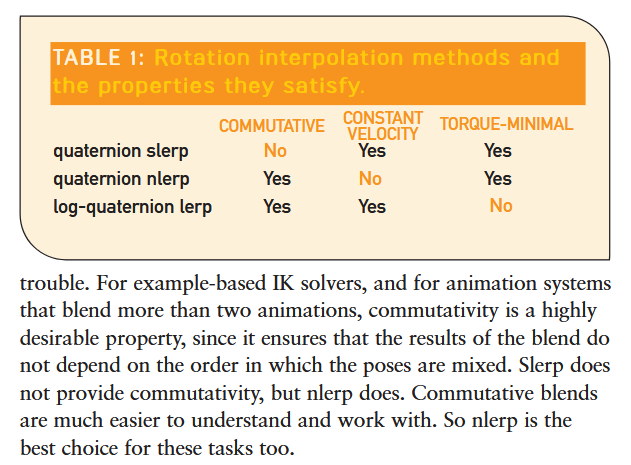Figure 20. Confusion in Game Developer Magazine.

There is a source of confusion that warrants a short discussion. In the previously mentioned Game Developer Magazine article, there is a quote (Figure 20) that pervades in conversations. "Slerp does not provide commutativity, but nlerp does."

which might be understood to mean that SLERP would be somehow inferior to NLERP.

The commonly held definition in mathematics is that when a binary operator `✲` is commutative [38], it means that `a✲b = b✲a`. In function notation, `OP(a,b) = OP(b,a)`. Scalar multiplication is commutative, matrix multiplication is not. Unlike what Game Developer Magazine stated, neither the SLERP nor the NLERP functions satisfy this. For example

NLERP(a,b,0) = a ≠ b = NLERP(b,a,0)

when `a≠b` just like `SLERP(a,b,0) ≠ SLERP(b,a,0)`.

Also, neither NLERP nor SLERP are associative operators [39]. An associative operator `✲` has the property that `(a✲b)✲c = a✲(b✲c)`, commonly meaning that "it doesn't matter where you put the parentheses."

For example, with notation `q = xi + yj + zk + w = (x, y, z, w)`, take

q0 = (0, 0, 0, 1)
q1 = (0, 0, sin 30°, cos 30°)
q2 = (0, 0, sin 90°, cos 90°)

i.e. q₀ is the identity orientation, q₁ rotation 60 degrees about the Z axis, and q₂ rotation 180 degrees about the Z axis.

Then,

NLERP(q0, NLERP(q1, q2, 1/2), 1/2) = (0, 0, sin 30°, cos 30°)
NLERP(NLERP(q0, q1, 1/2), q2, 1/2) = (0, 0, sin 52.5°, cos 52.5°)

⇒ NLERP(q0, NLERP(q1, q2, 1/2), 1/2) ≠ NLERP(NLERP(q0, q1, 1/2), q2, 1/2)

And likewise for SLERP, since at `t=1/2`, both NLERP and SLERP coincide (see Figure 1 in the beginning of the article). So in the context of 3D pose blending, for NLERP, the order in which poses are mixed matters just like it does for SLERP.

The NLERP and SLERP operators are not linear operators [40] in any of the arguments either. For a linear operator `L`, `L(ax + by) = aL(x) + bL(y)`. This property does not hold for either NLERP nor SLERP, i.e.

To set the record straight after all these years, what the author likely intended to communicate was that the weight re-biasing that the SLERP operator employs cannot be applied when there are more than two input orientations to blend together simultaneously. This is natural, since talking about constant velocity of travel for a single time parameterized value `t: 0 → 1` only applies in the formulation of SLERP when there are two endpoints.

When there are multiple inputs to blend between, with multiple weights, constant velocity parameterizations (under a suitable definition) will be more complicated to formulate than what SLERP for two inputs can offer. In such cases, the author's intention was probably to say that rather than try to find a constant velocity parameterization, it is simpler to do a weighted mix of all the input quaternions and normalize the result. I.e. to "NLERP" it all together.

It is important to not conflate different use cases. The fact that the traditional SLERP formulation only exists to operate on two input quaternions (although do see SQUAD from Shoemake 1987, pdf page 114 [41] and Appendix F) and not for more than two, does not mean that SLERP would be somehow defective for interpolating between two quaternions (and should not be bothered with). Because a car cannot fly, it does not mean that it wouldn't be good at driving on road.

So, when either SLERPing or NLERPing, be aware that there is no commutativity, associativity or linearity. The end points are not interchangeable, and both the normalization and the 4D dot product hemisphere re-flip steps prevent these properties from holding true.

It is possible that the Game Developer Magazine author was thinking of the pre-normalization step for `LERP90`. I.e. if we define for multiple input quaternions q_i and associated weights w_i and have `LERP90` and `NLERP90` take as input tuples of these elements, as in

where we restrict by some a priori construction that the input quaternions q_i are all guaranteed to be located on the same 4D hemisphere (or can mutually be ±q sign flipped to admit such collective configuration, or using `LERP90` makes arguably little sense), then `LERP90` is commutative and associative and linear (but does not produce a unit quaternion) and `NLERP90` is commutative, but not associative or linear. The order in which arguments are selected into `LERP90` and `NLERP90` functions is permutationally symmetric however.

The `NLERP90` function can be utilized in situations where multiple quaternions are weighed together, such that a constant velocity parameterization of two quaternions given by `SLERP` cannot be applied.

For the pedantic (e.g. maybe for developers writing unit test libraries), the formulations of SLERP and NLERP in this article all use the convention to flip the source quaternion to the 4D hemisphere of the destination. The following endpoint identities hence hold:

{N,S}LERP(a, b, 0) ≈ ±a
{N,S}LERP(a, b, 1) ≈ b

where `±a` means "returns either `a` or `-a`" (depending on `b`). The approximate equality `≈` is due to the normalization step, which will prevent bit exact return values.

Finally, both NLERP and SLERP have endpoint reversal symmetry:

{N,S}LERP(a, b, t) ≈ ±{N,S}LERP(b, a, 1-t)

where `±` denotes equivalence up to the sign, and midpoint symmetry:

{N,S}LERP(a, b, 1/2) ≈ ±normalize(±a+b)

Where `±a` denotes that the quaternion `a` is first flipped to the same 4D hemisphere of quaternion `b`.

Implementation Comparison

Optimizations to SLERP have been sought in the past. In chronological order, J.M.P. van Waveren wrote about a fast SLERP while at Id Software in 2005 ([42]). Their insight was to utilize a trigonometric identity to trade evaluation of the `acos()` function into an evaluation of `sqrt()` and `atan2()` functions, and apply the infamous Carmack inverse square root trick and a polynomial approximation to `sin()` and `atan2()`. In 2011 David Eberly applied the Chebyshev Equioscillation Theorem and Remez Algorithm for polynomial optimization to the whole numerator and denominator function expression of the weights ([6]), rather than the `sin()` and `acos()` functions separately in our presentation (Appendix G shows the approximation of `sin()` alone). The SLERP implementation in this article follows from the author's initial implementation in the open source MathGeoLib library that was developed in 2015 ([43]). Between 2015 and 2016 Arseny Kapoulkine ("Zeuxcg") published two SLERP approximations on their blog ([44], [45]). In 2019, a question by username "bzt" on the GameDev.net forum inspired Álvaro Begué ("alvaro") to suggest a fast approximation to SLERP ([46]).

In parallel, Tony Barrera, Anders Hast and Ewert Bengtsson proposed in 2004 ([47]) to optimize the computation of Incremental SLERP, i.e. exploiting a scenario of subdividing the SLERP rotation range into K equally spaced steps and sharing computation over each. In 2008, Mark Leeney improved on this scheme by applying de Moivre's identities to the incremental SLERP scheme ([48]). From our practical software engineering perspective, the benefit of the incremental SLERP scheme was seen situational so was not considered here further.

In this section, these different implementations are compared against the SSE version of our method presented in Listing 26, compiling to a native Windows executable using Clang version 24. Unlike the performance and error comparisons that were measured in WebAssembly in Figures 12, 13 and 14, the comparison against other SLERP methods in this chapter is done in native code to avoid unfair slowdown from emulated compilation of SSE in the browser in Eberly's presented code.

The original code presented by Eberly targeted the SSE1 instruction set only. To make a more modern performance comparison, Eberly's code was upgraded to utilize the newer SSE 4.1 + FMA instruction sets.

Estimating numerical precision requires careful analysis from multiple perspectives. As will be seen, there can exist numerical behavior to a particular SLERP implementation that can make it look good at first, but at the same time, exhibit behavior that breaks down in practical use in specific scenarios or code patterns. Therefore it is important to carefully enumerate different properties that a good SLERP function should have, and measure the numerical error in each of these. Only then can one have peace of mind that the numerical approximation is sound.

In the earlier section in Figures 13 and 14, the precision analysis compared the single-precision WebAssembly code against a double-precision JavaScript reference. However, for robust numerical analysis, that approach turns out to be disappointing for two main reasons. First, the reference implementation (Listing 4) computes in double-precision, so it is an approximation on its own, therefore unable to report numerical imprecision beyond the double precision computation limit. Second, the reference code from Listing 4 has a discontinuous `if (cosOmega >= 0.999)` test, where this exact cutoff constant `0.999` was rather arbitrarily selected.

To fix both of these errors, the numerical accuracy for the tests in this section were improved by using the Python `mpmath` package, computing "true" SLERP outputs over a hundred million random SLERPs using 100 digits of floating point precision, using the arithmetic reference formulation without discontinuities. This data was then rounded to double-precision and single-precision, to arrive at improved ground truth results that would be accurate up to a single ULP.

The code from van Waveren/Id Software contains two sources of undefined behavior and will need fixes to run correctly. The programming issues reside in the Carmack inverse square root function (Listing 20).

float ReciprocalSqrt(float x)
{
  // 'long' may be 64-bit on LP64 systems. Should use uint32_t instead of long.
  long i;
  float y, r;
  y = x * 0.5f;
  // Casting to long pointer breaks C strict aliasing rule. Either use standard
  // C memcpy() or e.g. LLVM/Clang `__builtin_bit_cast(uint32_t, x)` expression
  // or C++20 std::bit_cast().
  i = *(long *)(&x);
  i = 0x5f3759df - (i >> 1);
  // Ditto when casting back. Use memcpy() or `__builtin_bit_cast(float, i)` or
  // C++20 std::bit_cast().
  r = *(float *)(&i);
  r = r * (1.5f - r * r * y);
  return r;
}

After applying the fixes suggested in comments, the Carmack inverse square root function works as originally intended.

The different SLERP methods were tested using the following criteria.

• Instruction Count. This criteria measured the number of hot machine code instructions in each method. Lightweight assembly instructions such as MOVs, ADDs or SHUFFLEs were not calculated, since their overhead is generally diminishing. Transcendental functions were considered as one instruction. This calculation can give an approximate understanding to the overall performance of the method.
• Elapsed/call. Each method was microbenchmarked in a test harness, and the exact nanoseconds per individual SLERP call was measured. An AMD Ryzen 5950X CPU that was fixed to run at constant 3.4 GHz was used for benchmarking. The reader is advised to take microbenchmarking performance numbers with a grain of salt, as they represent synthetic esults.
• Max (ΔError)². For each Slerp output quaternion q_approx, the squared distance to the expected reference output q_ref can be calculated. Precisely, this calculation was done by first flipping both quaternions to the same 4D hemisphere, and then calculating the maximum `(ΔError)² := |q<sub>approx</sub> - q<sub>ref</sub>|²` over all the test input quaternions.
• Max Angular error. Another way to look at the error between the true and reference slerp output is to measure the angle between the two. In this error metric, the number of degrees that the approximated orientation should still need to be rotated to coincide with the ground truth expected orientation was measured. I.e. `Angular error := radToDeg(2cos⁻¹(|q<sub>approx</sub>·q<sub>ref</sub>|))`. This is the single most important error metric, as it measures how far away visually the SLERP implementation may drift from the true rotation result.
• Max (Norm Error)². The slerp output is expected to be a unit quaternion (since only unit quaternions represent pure rotations). 3D graphics calculations are generally able to sustain a small amount of divergence from unit length, but ideally the output should be as close to normalized as possible. This metric reports the maximum squared divergence of output quaternion length over all input quaternions. `|Norm Error|² := | |q<sub>approx</sub>|² - 1|.`
• Iteration error. Some use cases call for repeated iteration of SLERP on the slerp output vector, feeding the output back into as (a start/endpoint) input to a subsequent SLERP, and iterating this type of feedback several times. For example, when calculating a series of quaternion SLERPs for example inside an orientation solver, stability under iteration is critical. This metric reports the maximum amount of deviation from unit norm that occurred when repeatedly iterating quaternions in this manner.
• Max Snap error. Finally, certain use cases may be algebraically sensitive to specific mathematical identities holding up with the SLERP algorithm. This error metric tests the different methods on how far they diverge from the endpoint identities (`SLERP(a, b, 0) ≈ ±a`, `SLERP(a, b, 1) ≈ b`) and midpoint symmetry (`SLERP(a, b, 1/2) ≈ ±normalize((±a+b)/2)`) over all tested input quaternions. For a lack of a better term, this error is called "snap error", to highlight the expectation that at these special `t` values, the result should snap precisely to the arithmetic identity.

The results of these comparisons are shown in Figure 21.

To establish an understanding of the accuracy limits of double-precision and single precision computation, the original reference methods are presented at the top of the table (rows 0a and 0b). These versions call the accurate trigonometric functions from a system library. The reference SLERP is about 10x slower than the fast SSE NLERP (row 9).

The SLERP methods in the table are sorted in chronological order. Van Waveren's method (row 1) should not be considered current anymore. Their claim "[...] two times faster than linear interpolation with renormalization (Lerp) in C" no longer holds up on modern hardware, as their slerp is actually 5x slower than our NLERP. The use of the Carmack inverse square root results in failed numerical precision across the board, including catastrophic divergence from unit norm under iteration.

Eberly's code (row 2) and its SSE4.1 update (row 3) suffers from higher maximum angular error than our method and also since their method does not contain a quaternion renormalization step in the end, the maximum error with output norm is rather high and their method is not stable under iteration.

The iteration stability is easily restored in Eberly's code by adding a MUL+DIV+SQRT normalization in the end (row 4) and this gives it a great boost in precision, but that unfortunately causes a noticeable loss in overall performance.

Out of Arseny Kapoulkine's variants, the `onlerp` function (row 5) has good precision comparable to ours, but it is almost twice as slow than our method. The `fnlerp` variant (row 6) is faster, but accuracy, especially in the max angular error, suffers. Kapoulkine implements aggressive SIMD optimization to this method that invokes SLERP on four quaternions at a time, using the Structure of Arrays (SoA) method. That optimization effectively results in a perfect 4-fold performance increase compared to the numbers presented here. However it also requires substantial refactoring to the codebase.

Finally, Álvaro Begué's suggested variant (row 7) is a tiny bit more accurate than `fnlerp`, but has the same issue about norm drift as Eberly and van Waveren's methods have.

Our method (row 8) holds up on all tested metrics. It is the fastest and executes close to the SSE optimized NLERP (row 9) speed. Max angular error is 0.0749°, which is a tiny bit better even than the angular error in the single-precision reference implementation in C, likely due to help from FMA instructions. Since our method has an explicit normalization step, there is a guarantee that the norm will not drift. The Max (ΔError)² metric is not best in the pack, but still well within tolerance of visually indistinguishable results.

Disassembly and size analysis

The compiled WebAssembly code of the final slerp function can be disassembled with `wasm-objdump` into a linear WebAssembly opcode form. (Listing 21)

0002f5 func[15] <slerp>:
 0002f6: 01 7b                      | local[3] type=v128
 0002f8: 20 01                      | local.get 1
 0002fa: 20 00                      | local.get 0
 0002fc: 20 01                      | local.get 1
 0002fe: fd e6 01                   | f32x4.mul
 000301: 22 01                      | local.tee 1
 000303: 20 01                      | local.get 1
 000305: 20 01                      | local.get 1
 000307: fd 0d 04 05 06 07 00 01 02 | i8x16.shuffle 0x07060504 0x03020100 0x0f0e0d0c 0x0b0a0908
 000310: 03 0c 0d 0e 0f 08 09 0a 0b | 
 000319: fd e4 01                   | f32x4.add
 00031c: 22 01                      | local.tee 1
 00031e: 20 01                      | local.get 1
 000320: 20 01                      | local.get 1
 000322: fd 0d 08 09 0a 0b 0c 0d 0e | i8x16.shuffle 0x0b0a0908 0x0f0e0d0c 0x03020100 0x07060504
 00032b: 0f 00 01 02 03 04 05 06 07 | 
 000334: fd e4 01                   | f32x4.add
 000337: 22 03                      | local.tee 3
 000339: fd e0 01                   | f32x4.abs
 00033c: 22 01                      | local.tee 1
 00033e: fd 0c da 2a be be da 2a be | v128.const 0xbebe2ada 0xbebe2ada 0xbebe2ada 0xbebe2ada
 000347: be da 2a be be da 2a be be | 
 000350: fd 0c d2 d2 f0 3d d2 d2 f0 | v128.const 0x3df0d2d2 0x3df0d2d2 0x3df0d2d2 0x3df0d2d2
 000359: 3d d2 d2 f0 3d d2 d2 f0 3d | 
 000362: fd 85 02                   | f32x4.relaxed_madd
 000365: 20 01                      | local.get 1
 000367: fd 0c 25 ca 82 bf 25 ca 82 | v128.const 0xbf82ca25 0xbf82ca25 0xbf82ca25 0xbf82ca25
 000370: bf 25 ca 82 bf 25 ca 82 bf | 
 000379: fd 85 02                   | f32x4.relaxed_madd
 00037c: 20 01                      | local.get 1
 00037e: fd 0c 79 23 c9 3f 79 23 c9 | v128.const 0x3fc92379 0x3fc92379 0x3fc92379 0x3fc92379
 000387: 3f 79 23 c9 3f 79 23 c9 3f | 
 000390: fd 85 02                   | f32x4.relaxed_madd
 000393: 20 03                      | local.get 3
 000395: fd 0c 00 00 00 80 00 00 00 | v128.const 0x80000000 0x00000000 0x00000000 0x00000000
 00039e: 00 00 00 00 00 00 00 00 00 | 
 0003a7: fd 4e                      | v128.and
 0003a9: fd 0c 00 00 00 00 00 00 00 | v128.const 0x00000000 0x00000000 0x00000000 0x00000000
 0003b2: 00 00 00 00 00 00 00 00 00 | 
 0003bb: 43 00 00 80 3f             | f32.const 0x1p+0
 0003c0: 20 02                      | local.get 2
 0003c2: 93                         | f32.sub
 0003c3: fd 20 00                   | f32x4.replace_lane 0
 0003c6: 20 02                      | local.get 2
 0003c8: fd 20 01                   | f32x4.replace_lane 1
 0003cb: fd 51                      | v128.xor
 0003cd: fd e6 01                   | f32x4.mul
 0003d0: 22 01                      | local.tee 1
 0003d2: 20 01                      | local.get 1
 0003d4: 20 01                      | local.get 1
 0003d6: fd e6 01                   | f32x4.mul
 0003d9: 22 01                      | local.tee 1
 0003db: fd 0c 2a 3b f6 3b 2a 3b f6 | v128.const 0x3bf63b2a 0x3bf63b2a 0x3bf63b2a 0x3bf63b2a
 0003e4: 3b 2a 3b f6 3b 2a 3b f6 3b | 
 0003ed: 20 01                      | local.get 1
 0003ef: fd 0c 34 a6 29 be 34 a6 29 | v128.const 0xbe29a634 0xbe29a634 0xbe29a634 0xbe29a634
 0003f8: be 34 a6 29 be 34 a6 29 be | 
 000401: fd 85 02                   | f32x4.relaxed_madd
 000404: fd 0c 21 ec 7f 3f 21 ec 7f | v128.const 0x3f7fec21 0x3f7fec21 0x3f7fec21 0x3f7fec21
 00040d: 3f 21 ec 7f 3f 21 ec 7f 3f | 
 000416: fd 85 02                   | f32x4.relaxed_madd
 000419: fd e6 01                   | f32x4.mul
 00041c: 22 01                      | local.tee 1
 00041e: 20 01                      | local.get 1
 000420: fd 0d 04 05 06 07 04 05 06 | i8x16.shuffle 0x07060504 0x07060504 0x07060504 0x07060504
 000429: 07 04 05 06 07 04 05 06 07 | 
 000432: 20 00                      | local.get 0
 000434: 20 01                      | local.get 1
 000436: 20 01                      | local.get 1
 000438: fd 0d 00 01 02 03 00 01 02 | i8x16.shuffle 0x03020100 0x03020100 0x03020100 0x03020100
 000441: 03 00 01 02 03 00 01 02 03 | 
 00044a: fd e6 01                   | f32x4.mul
 00044d: fd 85 02                   | f32x4.relaxed_madd
 000450: 22 00                      | local.tee 0
 000452: 20 00                      | local.get 0
 000454: 20 00                      | local.get 0
 000456: fd e6 01                   | f32x4.mul
 000459: 22 00                      | local.tee 0
 00045b: 20 00                      | local.get 0
 00045d: 20 00                      | local.get 0
 00045f: fd 0d 04 05 06 07 00 01 02 | i8x16.shuffle 0x07060504 0x03020100 0x0f0e0d0c 0x0b0a0908
 000468: 03 0c 0d 0e 0f 08 09 0a 0b | 
 000471: fd e4 01                   | f32x4.add
 000474: 22 00                      | local.tee 0
 000476: 20 00                      | local.get 0
 000478: 20 00                      | local.get 0
 00047a: fd 0d 08 09 0a 0b 0c 0d 0e | i8x16.shuffle 0x0b0a0908 0x0f0e0d0c 0x03020100 0x07060504
 000483: 0f 00 01 02 03 04 05 06 07 | 
 00048c: fd e4 01                   | f32x4.add
 00048f: fd e3 01                   | f32x4.sqrt
 000492: fd e7 01                   | f32x4.div
 000495: 0b                         | end

The disassembly highlights are

• 1 vector square root (`f32x4.sqrt`)
• 1 vector division (`f32x4.div`)
• 12 vector multiplications (6 `f32x4.mul`, 6 `f32x4.relaxed_madd`)

which generate 417 bytes of branch-free code in total.

Observing the assembly code does make one ponder whether more size efficient Wasm SIMD encodings for some SIMD operations (e.g. i32x4.splat or i32x4.shuffle) might help improve WebAssembly code density.

Node.js has the useful `--print-wasm-code` and `--print-wasm-code-function-index=<N>` command line flags which enable examining the generated native CPU assembly. Given that this same code is presented in both optimized native SSE (Appendix D) and in WebAssembly SIMD (Appendix A), there is a unique opportunity to compare the native Clang compiler Intel x64 SSE assembly against TurboFan compiled Intel x64 SSE code. A core promise of the WebAssembly standard is to enable computation at native level of performance, modulo the security sandboxing that is required for safe web computing.

The comparison between native Clang compiler and the V8 TurboFan optimizing compiler is presented side by side in Listing 22.

; // 1) cosOmega = dot(from, to)                       | ; // 1) cosOmega = dot(from, to)
;  __m128 cosOmega = _mm_dp_ps(from, to, 0xFF);        | ;  __f32x4 cosOmega = dp(from, to);
                                                       | 
   vdpps xmm2, xmm0, xmm1, 0xff                        |    vmulps xmm0,xmm1,xmm2
                                                       |    vpshufd xmm4,xmm0,0xb1
                                                       |    vaddps xmm0,xmm0,xmm4
                                                       |    vpshufd xmm4,xmm0,0x4e
                                                       |    vaddps xmm0,xmm0,xmm4
                                                       | 
; // 2) w = [1-t, t, 0, 0], negated if cosOmega < 0    | ; // 2) w = [1-t, t, 0, 0], negated if cosOmega < 0
;  __m128 w = _mm_xor_ps(_mm_set_ps(0, 0, t, 1-t),     | ;  __f32x4 w = v128_xor(f32x4_make(1-t, t, 0, 0),
;    _mm_and_ps(cosOmega, _mm_set_ss(-0.0f)));         | ;  v128_and(cosOmega, i32x4_make(0x80000000u,0,0,0)));
                                                       | 
   vmovss  xmm3, dword ptr [r15 + 4*r8]                |    vpcmpeqd xmm5,xmm5,xmm5
   vsubss  xmm4, xmm10, xmm3                           |    vpsllq xmm5,xmm5,63
   vinsertps xmm3, xmm4, xmm3, 0x1c                    |    vpsrlq xmm5,xmm5,32
   vandps  xmm4, xmm13, xmm2                           |    REX.W movq r10,0000000000000000
   vxorps  xmm3, xmm4, xmm3                            |    vpinsrq xmm5,xmm5,r10,0x1    
                                                       |    vpand xmm0,xmm0,xmm5         
                                                       |    vpxor xmm5,xmm5,xmm5         
                                                       |    vpcmpeqd xmm6,xmm6,xmm6      
                                                       |    vpslld xmm6,xmm6,25          
                                                       |    vpsrld xmm6,xmm6,2           
                                                       |    vsubss xmm6,xmm6,xmm3        
                                                       |    vinsertps xmm5,xmm5,xmm6,0x0 
                                                       |    vinsertps xmm5,xmm5,xmm3,0x10
                                                       |    vpxor xmm0,xmm0,xmm5         
                                                       | 
; // 3) acos polynomial                                | ; // 3) acos polynomial
;  __m128 x = _mm_and_ps(cosOmega, _mm_castsi128_ps(   |
;                        _mm_set1_epi32(0x7fffffff))); | ;  __f32x4 x = f32x4_abs(cosOmega);
                                                       | 
   vandps  xmm2, xmm9, xmm2                            |    REX.W movq r10,00007FF7F7D684A0
                                                       |    vandps xmm4,xmm0,[r10]
                                                       | 
;  __m128 ang = _mm_fmadd_ps(x, -0.371..., 0.117...);  | ;  __f32x4 a = f32x4_relaxed_madd(x, 
;  ang = _mm_fmadd_ps(ang, x, -1.021...);              | ;    -0.371..., 0.117...);
;  ang = _mm_fmadd_ps(ang, x,  1.571...);              | ;  a = f32x4_relaxed_madd(a, x, -1.021...);
                                                       | ;  a = f32x4_relaxed_madd(a, x,  1.571...);
                                                       | 
  vmovaps xmm4, xmm7                                   |    REX.W movq r10,BEBE2ADABEBE2ADA
  vfmadd213ps xmm4, xmm2, xmm11                        |    vmovq xmm5,r10
  vfmadd213ps xmm4, xmm2, xmmword ptr [rip + 0x22148]  |    vpunpcklqdq xmm5,xmm5,xmm5
  vfmadd213ps xmm4, xmm2, xmmword ptr [rip + 0x2214f]  |    REX.W movq r10,3DF0D2D23DF0D2D2
                                                       |    vmovq xmm6,r10
                                                       |    vpunpcklqdq xmm6,xmm6,xmm6
                                                       |    vfmadd213ps xmm5,xmm4,xmm6
                                                       |    REX.W movq r10,BF82CA25BF82CA25
                                                       |    vmovq xmm6,r10
                                                       |    vpunpcklqdq xmm6,xmm6,xmm6
                                                       |    vfmadd213ps xmm5,xmm4,xmm6
                                                       |    REX.W movq r10,3FC923793FC92379
                                                       |    vmovq xmm6,r10
                                                       |    vpunpcklqdq xmm6,xmm6,xmm6
                                                       |    vfmadd213ps xmm4,xmm5,xmm6
                                                       | 
;  w = _mm_mul_ps(w, ang);                             | ;  w = f32x4_mul(w, a);
   vmulps  xmm2, xmm4, xmm3                            |    vmulps xmm0,xmm4,xmm0
                                                       | 
; // 4) sin polynomial applied to w                    | ; // 4) sin polynomial applied to w
;  __m128 xx = _mm_mul_ps(w, w);                       | ;  __f32x4 xx = f32x4_mul(w, w);
   vmulps  xmm3, xmm2, xmm2                            |    vmulps xmm3,xmm0,xmm0
                                                       | 
;  __m128 a = _mm_fmadd_ps(xx, 0.007..., -0.165...);   | ;  __f32x4 a = f32x4_relaxed_madd(
;  a = _mm_fmadd_ps(a, xx, 0.999...);                  | ;    0.007..., xx, -0.165...);
   vmovaps xmm4, xmm8                                  | ;  a = f32x4_relaxed_madd(xx, a, 0.999...);
   vfmadd213ps xmm4, xmm3, xmmword ptr [rip + 0x2214a] |    REX.W movq r10,3BF63B2A3BF63B2A
   vfmadd213ps xmm4, xmm3, xmmword ptr [rip + 0x22151] |    vmovq xmm4,r10
                                                       |    vpunpcklqdq xmm4,xmm4,xmm4
                                                       |    REX.W movq r10,BE29A634BE29A634
                                                       |    vmovq xmm5,r10
                                                       |    vpunpcklqdq xmm5,xmm5,xmm5
                                                       |    vfmadd213ps xmm4,xmm3,xmm5
                                                       |    REX.W movq r10,3F7FEC213F7FEC21
                                                       |    vmovq xmm5,r10
                                                       |    vpunpcklqdq xmm5,xmm5,xmm5
                                                       |    vfmadd213ps xmm3,xmm4,xmm5
                                                       | 
;  w = _mm_mul_ps(w, _mm_fmadd_ps(xx, a, 0.999...));   | ;  w = f32x4_mul(w, a);
   vmulps  xmm2, xmm2, xmm4                            |    vmulps xmm0,xmm0,xmm3
                                                       | 
; // 5) ret = from*w0 + to*w1                          | ; // 5) ret = from*w0 + to*w1
;  __m128 ret = _mm_mul_ps(from,                       | ;  __f32x4 ret = f32x4_mul(from, 
;    _mm_shuffle_ps(w, w, _MM_SHUFFLE(0,0,0,0)));      | ;    i32x4_shuffle(w,w,0,0,0,0));
   vshufps xmm3, xmm2, xmm2, 0x0                       |    vpshufd xmm3,xmm0,0x55
   vmulps  xmm0, xmm0, xmm3                            |    vpshufd xmm0,xmm0,0x0
                                                       |    vmulps xmm0,xmm1,xmm0
                                                       | 
;  ret = _mm_fmadd_ps(to,                              | ;  ret = f32x4_relaxed_madd(to,
;    _mm_shuffle_ps(w, w, _MM_SHUFFLE(1,1,1,1)), ret); | ;    i32x4_shuffle(w,w,1,1,1,1), ret);
   vshufps xmm2, xmm2, xmm2, 0x55                      |    vfmadd231ps xmm0,xmm3,xmm2
   vfmadd213ps xmm2, xmm1, xmm0                        | 
                                                       | 
; // 6) renormalize: ret = ret / |ret|                 | ; // 6) renormalize: ret = ret / |ret|
;  return _mm_div_ps(ret,                              | ;  return f32x4_div(ret, f32x4_sqrt(dp(ret, ret)));
;    _mm_sqrt_ps(_mm_dp_ps(ret, ret, 0xFF)));          | 
   vdpps   xmm0, xmm2, xmm2, 0xff                      |    vmulps xmm2,xmm0,xmm0
   vsqrtps xmm0, xmm0                                  |    vpshufd xmm3,xmm2,0xb1
   vdivps  xmm0, xmm2, xmm0                            |    vaddps xmm2,xmm2,xmm3
                                                       |    vpshufd xmm3,xmm2,0x4e
                                                       |    vaddps xmm2,xmm2,xmm3
                                                       |    vsqrtps xmm2,xmm2
                                                       |    vdivps xmm1,xmm0,xmm2

The V8 generated code does indeed utilize the same native hardware SSE `vfmadd213ps` instructions, but it does look like there are shortcomings in the V8 code generation, namely:

1. `Blocks 1 and 6`: Lack of support for the `dpps` instruction (and the `haddps` instruction) result in a pessimized `vmulps+vpshufd+vaddps+vpshufd+vaddps` stream of instructions.
2. `Block 2`: Lack of access to scalar computation inside the SSE registers (`vmovss+vsubss`) result in a longer code to set up the `w = [1-t, t, 0, 0]` vector.
3. `Blocks 3 and 4`: SIMD constants (via `wasm_f32x4_splat()`) utilize a more inefficient sequence of `movq+vmovq+vpunpcklqdq` instructions in V8, rather than access the constants directly from memory.

The limitations 1 and 2 are result of a design choice in WebAssembly SIMD, where the intent was to not expose the native SIMD instruction capabilities in the API.

The limitation 3 seems to be a behavior of the V8 TurboFan compiler and could possibly be optimized in a later release.

These differences together explain why the SLERP function performance was seen to run more than twice as slow in Figure 12 when measured in WebAssembly SIMD, when compared to running in native SSE in Figure 21.

Conclusion

A branch-free and system library trigonometric function free construction of the SLERP algorithm was presented that utilizes WebAssembly 3.0 FMA instructions. The function benchmarks to about 36.4 ns/call in the browser on an AMD 5950X CPU, has a max square deviation of 3.6e-8 and a max orientation angle error of ≈ 0.0749° degrees. Disk size footprint is 417 bytes (uncompressed) with 75 WebAssembly opcodes.

The majority of performance improvement was gained by replacing the standard library's trigonometric function calls with inline approximations that are tuned for real-time computation and the total error of the slerp function, rather than using accurate precision transcendentals intended for data science.

References

1. "WebAssembly 3.0", WebAssembly Community Group announcement, September 2025.
2. "Quaternion", Wikipedia. https://en.wikipedia.org/wiki/Quaternion
3. Erik B. Dam, Martin Koch, Martin Lillholm, "Quaternions, Interpolation and Animation", Technical Report DIKU-TR-98/5, Department of Computer Science, University of Copenhagen, 1998. (local copy: QuaternionReport1.pdf)
4. Jim Van Verth, "Math for Game Programmers: Understanding Quaternions", Game Developers Conference (GDC) 2013. https://gdcvault.com/play/1017653/Math-for-Game-Programmers-Understanding
5. "The Unnecessarily Short Ways to do a Quaternion Slerp", Magnum Graphics blog. https://blog.magnum.graphics/backstage/the-unnecessarily-short-ways-to-do-a-quaternion-slerp/
6. David Eberly, "A Fast and Accurate Estimate for SLERP", Geometric Tools, 2018. (local copy: FastAndAccurateSlerp.pdf)
7. KhronosGroup/glTF-Sample-Models issue #185. https://github.com/KhronosGroup/glTF-Sample-Models/issues/185
8. Ken Shoemake, "Animating Rotation with Quaternion Curves", SIGGRAPH 1985, Computer Graphics, vol. 19, no. 3. (local copy: p245-shoemake.pdf)
9. Eric Lengyel, "Mathematics for 3D Game Programming and Computer Graphics, Third Edition", Chapter 4.6.3, Charles River Media, 2012.
10. LLVM/Clang, `<wasm_simd128.h>` WebAssembly SIMD intrinsics header. https://github.com/llvm/llvm-project/blob/main/clang/lib/Headers/wasm_simd128.h
11. Emscripten documentation, "Compiling SIMD code targeting X86 SSE instruction sets". https://emscripten.org/docs/porting/simd.html
12. WebAssembly Relaxed SIMD proposal, "Phase 4" ratification announcement, blink-dev mailing list, March 2023. https://groups.google.com/a/chromium.org/g/blink-dev/c/HzLlEGLSx7E
13. Can I use, "WebAssembly: relaxed-simd" browser compatibility table. https://caniuse.com/mdn-webassembly_relaxed-simd
14. WebAssembly Relaxed SIMD proposal overview. https://github.com/WebAssembly/relaxed-simd/blob/main/proposals/relaxed-simd/Overview.md
15. "Slerp demystified", Unity community discussion, 2022. https://discussions.unity.com/t/slerp-demystified/892580/2
16. Epic Games, Unreal Engine 4, `FQuat::Slerp` in UnrealMath.cpp. https://github.com/EpicGames/UnrealEngine/blob/f509bb2d6c62806882d9a10476f3654cf1ee0634/Engine/Source/Runtime/Core/Private/Math/UnrealMath.cpp#L1198
17. mrdoob/three.js, `Quaternion.slerp()` in src/math/Quaternion.js. https://github.com/mrdoob/three.js/blob/ad005397bbd15b0a9fcd5159c782eba56e1cba2a/src/math/Quaternion.js#L47-L129
18. g-truc/glm, `glm::slerp()` in glm/ext/quaternion_common.inl. https://github.com/g-truc/glm/blob/6f14f4792a0cde5d0cf2c910506724d61cb95834/glm/ext/quaternion_common.inl#L40-L73
19. Unity documentation, `Quaternion.Lerp`. https://docs.unity3d.com/6000.0/Documentation/ScriptReference/Quaternion.Lerp.html
20. Jacco Bikker, "Practical SIMD Programming", Universiteit Utrecht course material. (local copy: SIMD tutorial.pdf)
21. Moreno Marzolla, "SIMD Programming", Università di Bologna course material. (local copy: SIMD.pdf)
22. "Taylor series" (Maclaurin series of common functions), Wikipedia. https://en.wikipedia.org/wiki/Taylor_series
23. "Equioscillation theorem", Wikipedia. https://en.wikipedia.org/wiki/Equioscillation_theorem
24. Intel Intrinsics Guide. https://www.intel.com/content/www/us/en/docs/intrinsics-guide/index.html
25. "Horner's method", Wikipedia. https://en.wikipedia.org/wiki/Horner%27s_method
26. "Unit in the last place", Wikipedia. https://en.wikipedia.org/wiki/Unit_in_the_last_place
27. MDN Web Docs, `Math.fround()`. https://developer.mozilla.org/en-US/docs/Web/JavaScript/Reference/Global_Objects/Math/fround
28. Jonathan Blow, "Understanding Slerp, Then Not Using It", Game Developer Magazine, April 2004. (local copy: GDM_April_2004.pdf)
29. "(300) Math for Programmers: Physics", Game Developers Conference (GDC). https://gdcvault.com/play/1645/(300)-Math-for-Programmers-Physics
30. "three.js Quaternion.slerp gives bad result near poles", Stack Overflow question. https://stackoverflow.com/questions/56162239
31. ShaderToy shader 4tdGWB.
32. ShaderToy shader 7dKBzd.
33. Donald Knuth's optimization quote, as collected by The Laws of Software. https://www.laws-of-software.com/laws/knuth/
34. "Fast inverse square root", Wikipedia. https://en.wikipedia.org/wiki/Fast_inverse_square_root
35. Khronos Group, glTF 2.0 specification, section "Animation Sampler Interpolation". https://registry.khronos.org/glTF/specs/2.0/glTF-2.0.html
36. KhronosGroup/glTF issue #1395. https://github.com/KhronosGroup/glTF/issues/1395
37. Unity documentation, Unity.Mathematics.math.nlerp. https://docs.unity3d.com/Packages/com.unity.mathematics@1.3/api/Unity.Mathematics.math.nlerp.html
38. "Commutative property", Wikipedia. https://en.wikipedia.org/wiki/Commutative_property
39. "Associative property", Wikipedia. https://en.wikipedia.org/wiki/Associative_property
40. "Linear map", Wikipedia. https://en.wikipedia.org/wiki/Linear_map
41. David Sturman et al. (eds.), "Computer Animation: 3-D Motion Specification and Control" (including Ken Shoemake's SQUAD presentation), SIGGRAPH 1987 Course Notes. (local copy: 102724883-05-10-acc.pdf)
42. J.M.P. van Waveren, "SIMD Slerping Clock Cycles" (fast SLERP at Id Software), 2005. (local copy: SIMD-Slerping-Clock-Cycles.pdf)
43. Jukka Jylänki, MathGeoLib initial SLERP implementation commit, 2015. https://github.com/juj/MathGeoLib/commit/e40e9a5451ddfecb59206b8d084d54c02d0c9317
44. Arseny Kapoulkine ("Zeuxcg"), "Approximating slerp", Zeux.io blog, 2015. https://zeux.io/2015/07/23/approximating-slerp/
45. Arseny Kapoulkine ("Zeuxcg"), "Optimizing slerp", Zeux.io blog, 2016. https://zeux.io/2016/05/05/optimizing-slerp/
46. Álvaro Begué ("alvaro"), reply in the "Optimized slerp" forum thread, GameDev.net, 2019. https://gamedev.net/forums/topic/704482-optimized-slerp/5415975/
47. Tony Barrera, Anders Hast, Ewert Bengtsson, "Incremental Spherical Linear Interpolation", 2004. (local copy: ecp01304.pdf)
48. Mark Leeney, "Fast quaternion slerp", International Journal of Computer Mathematics, vol. 86, no. 1, pp. 79-84, 2009. https://doi.org/10.1080/00207160801923064

Appendix A. WebAssembly code

Here is the completed WebAssembly 3.0 code.

#ifdef __wasm_relaxed_simd__

#include <wasm_simd128.h>

// Calculates dot product a·b into all lanes of the returned vector.
static __f32x4 dp(__f32x4 a, __f32x4 b)
{
  a = wasm_f32x4_mul(a, b);
  a = wasm_f32x4_add(a, wasm_i32x4_shuffle(a, a, 1, 0, 3, 2));
  return wasm_f32x4_add(a, wasm_i32x4_shuffle(a, a, 2, 3, 0, 1));
}

__f32x4 slerp(__f32x4 from, __f32x4 to, float t)
{
  __f32x4 cosOmega = dp(from, to);
  __f32x4 w = wasm_v128_xor(wasm_f32x4_make(1-t, t, 0, 0), wasm_v128_and(cosOmega, wasm_i32x4_make(0x80000000u,0,0,0))); 

  // acos
  __f32x4 x = wasm_f32x4_abs(cosOmega);
  __f32x4 a = wasm_f32x4_relaxed_madd(x, wasm_f32x4_splat(-0.627160617651148722f),
                                         wasm_f32x4_splat(0.366191412084127366f));
  a = wasm_f32x4_relaxed_madd(a, x, wasm_f32x4_splat(-1.06803417726155914f));
  a = wasm_f32x4_relaxed_madd(a, x, wasm_f32x4_splat(1.57316997572997042f));
  w = wasm_f32x4_mul(w, a);

  // sin
  __f32x4 xx = wasm_f32x4_mul(w, w);
  a = wasm_f32x4_relaxed_madd(wasm_f32x4_splat(0.007514377178300066f), xx, wasm_f32x4_splat(-0.16567307932054615f));
  w = wasm_f32x4_mul(w, wasm_f32x4_relaxed_madd(xx, a, wasm_f32x4_splat(0.9996967731390435f)));

  // lerp
  __f32x4 ret = wasm_f32x4_mul(from, wasm_i32x4_shuffle(w,w,0,0,0,0));
  ret = wasm_f32x4_relaxed_madd(to, wasm_i32x4_shuffle(w,w,1,1,1,1), ret);

  // renormalize
  return wasm_f32x4_div(ret, wasm_f32x4_sqrt(dp(ret, ret)));
}
#endif

Compile with Emscripten flag `-mrelaxed-simd`.

Appendix B. Scalar C code

For use on platforms that do not support the needed SIMD code (e.g. embedded computing and the Safari browser), here is a portable scalarized C version of the SLERP function.

#include <math.h>

void slerp(float *dst, float *from, float *to, float t)
{
  float cosOmega = from[0]*to[0] + from[1]*to[1] + from[2]*to[2] + from[3]*to[3];

  float x = fabsf(cosOmega);

  // acos()
  float angle = x*(x*(x*-0.627160617651148722f + 0.366191412084127366f) - 1.06803417726155914f) + 1.57316997572997042f;

  // Lerp weights
  float a = 1 - t;
  float x0 = (cosOmega < 0 ? -a : a) * angle;
  float x1 = t * angle;

  // sin()
  float x0x0 = x0 * x0;
  float x1x1 = x1 * x1;
  float w0 = x0*(0.9996967731390435f + x0x0*(-0.16567307932054615f + 0.007514377178300066f*x0x0));
  float w1 = x1*(0.9996967731390435f + x1x1*(-0.16567307932054615f + 0.007514377178300066f*x1x1));

  // Lerp
  float ret[4];
  ret[0] = from[0]*w0 + to[0]*w1;
  ret[1] = from[1]*w0 + to[1]*w1;
  ret[2] = from[2]*w0 + to[2]*w1;
  ret[3] = from[3]*w0 + to[3]*w1;

  // Renormalize
  float inv = 1.f / sqrtf(ret[0]*ret[0] + ret[1]*ret[1] + ret[2]*ret[2] + ret[3]*ret[3]);
  dst[0] = ret[0]*inv;
  dst[1] = ret[1]*inv;
  dst[2] = ret[2]*inv;
  dst[3] = ret[3]*inv;
}

Note however that the original error analysis was performed for the SIMD variant that utilizes FMA instructions. Those have slightly different precision from scalar code, so the precision analysis does not apply 100% to this version.

Appendix C. JavaScript code

This section contains a JavaScript version of the code.

function slerp(from, to, t) {
  var cosOmega = from.x*to.x + from.y*to.y + from.z*to.z + from.w*to.w;

  var x = Math.abs(cosOmega);

  // acos()
  var angle = x*(x*(x*-0.627160617651148722 + 0.366191412084127366) - 1.06803417726155914) + 1.57316997572997042;

  // Lerp weights
  var a = 1 - t;
  var x0 = (cosOmega < 0 ? -a : a) * angle;
  var x1 = t * angle;

  // sin()
  var x0x0 = x0 * x0;
  var x1x1 = x1 * x1;
  var w0 = x0*(0.9996967731390435 + x0x0*(-0.16567307932054615 + 0.007514377178300066*x0x0));
  var w1 = x1*(0.9996967731390435 + x1x1*(-0.16567307932054615 + 0.007514377178300066*x1x1));

  // Lerp
  var rx = from.x*w0 + to.x*w1;
  var ry = from.y*w0 + to.y*w1;
  var rz = from.z*w0 + to.z*w1;
  var rw = from.w*w0 + to.w*w1;

  // Renormalize
  var inv = 1 / Math.sqrt(rx*rx + ry*ry + rz*rz + rw*rw);

  return {
    x: rx * inv,
    y: ry * inv,
    z: rz * inv,
    w: rw * inv 
  }
}

Be mindful of temporary object allocation in the end and refer to the memory allocation profiler to see whether object pooling could be beneficial, or consider using a large Float32Array-based table representation for quaternions (and vectors and matrices).

Appendix D. Intel SSE code

The WebAssembly SIMD code translates well to the Intel SSE intrinsics set.

#if defined(__SSE4_1__) && defined(__FMA__)

#include <xmmintrin.h>
#include <emmintrin.h>
#include <smmintrin.h>
#include <immintrin.h>

__m128 slerp(__m128 from, __m128 to, float t)
{
  __m128 cosOmega = _mm_dp_ps(from, to, 0xFF);
  __m128 w = _mm_xor_ps(_mm_set_ps(0, 0, t, 1-t), _mm_and_ps(cosOmega, _mm_set_ss(-0.f)));
  __m128 x = _mm_and_ps(cosOmega, _mm_castsi128_ps(_mm_set1_epi32(0x7fffffff)));

  // acos
  __m128 ang = _mm_fmadd_ps(x, _mm_set1_ps(-0.627160617651148722f), _mm_set1_ps(0.366191412084127366f));
  ang = _mm_fmadd_ps(ang, x, _mm_set1_ps(-1.06803417726155914f));
  ang = _mm_fmadd_ps(ang, x, _mm_set1_ps(1.57316997572997042f));
  w = _mm_mul_ps(w, ang);

  // sin
  __m128 xx = _mm_mul_ps(w, w);
  __m128 a  = _mm_fmadd_ps(xx, _mm_set1_ps(0.007514377178300066f), _mm_set1_ps(-0.16567307932054615f));
  w = _mm_mul_ps(w, _mm_fmadd_ps(xx, a, _mm_set1_ps(0.9996967731390435f)));

  // lerp
  __m128 ret = _mm_mul_ps(from, _mm_shuffle_ps(w, w, _MM_SHUFFLE(0,0,0,0)));
  ret = _mm_fmadd_ps(to, _mm_shuffle_ps(w, w, _MM_SHUFFLE(1,1,1,1)), ret);

  // renormalize
  return _mm_div_ps(ret, _mm_sqrt_ps(_mm_dp_ps(ret, ret, 0xFF)));
}

#endif

This code should be compiled with `-msse4.1 -mfma` in GCC and LLVM/Clang.

Appendix E. Arm NEON code

On the ARM instruction set, the following NEON targeting code can be used.

#if defined(__aarch64__)

#include <arm_neon.h>

float32x4_t slerp(float32x4_t from, float32x4_t to, float t)
{
  float32x4_t cosOmega = vdupq_n_f32(vaddvq_f32(vmulq_f32(from, to)));
  float32x4_t w = { 1-t, t, 0, 0 };
  uint32x4_t sign = vandq_u32(vreinterpretq_u32_f32(cosOmega), (uint32x4_t){ 0x80000000u, 0, 0, 0 });
  w = vreinterpretq_f32_u32(veorq_u32(vreinterpretq_u32_f32(w), sign));
  float32x4_t x = vabsq_f32(cosOmega);

  // acos
  float32x4_t ang = vfmaq_f32(vdupq_n_f32(0.366191412084127366f), x, vdupq_n_f32(-0.627160617651148722f));
  ang = vfmaq_f32(vdupq_n_f32(-1.06803417726155914f), ang, x);
  ang = vfmaq_f32(vdupq_n_f32(1.57316997572997042f), ang, x);
  w = vmulq_f32(w, ang);

  // sin
  float32x4_t xx = vmulq_f32(w, w);
  float32x4_t a  = vfmaq_f32(vdupq_n_f32(-0.16567307932054615f), xx, vdupq_n_f32(0.007514377178300066f));
  w = vmulq_f32(w, vfmaq_f32(vdupq_n_f32(0.9996967731390435f), xx, a));

  // lerp
  float32x4_t ret = vmulq_f32(from, vdupq_laneq_f32(w, 0));
  ret = vmlaq_f32(ret, to, vdupq_laneq_f32(w, 1));

  // renormalize
  return vdivq_f32(ret, vsqrtq_f32(vdupq_n_f32(vaddvq_f32(vmulq_f32(ret, ret)))));
}

#endif

Appendix F. Optimized SQUAD interpolation

The final SIMD optimized SLERP implementation enables a fantastic follow-up optimization that two SLERPs can be computed in parallel.

The Spherical Quadrangle Interpolation (SQUAD) algorithm (Shoemake 1987, pdf page 114), which is used for example in the animation specification of the GLTF file standard, involves two sub-evaluations of SLERP at once.

SQUAD(𝑝,𝑎,𝑏,𝑞;t) = SLERP(SLERP(𝑝,𝑞;t),
                         SLERP(𝑎,𝑏;t);
                         2*⁢(1−t)*⁢t)

The structure of our optimized SIMD SLERP extends really well for this. We can fuse the computation of `SLERP(𝑝,𝑞;t)` and `SLERP(𝑎,𝑏;t)` into one.

// Calculates two dot products simultaneously (a·b, a·b, x·y, x·y)
static __f32x4 dp2(__f32x4 a, __f32x4 b, __f32x4 x, __f32x4 y)
{
  a = wasm_f32x4_mul(a, b);
  x = wasm_f32x4_mul(x, y);
  a = wasm_f32x4_add(wasm_i32x4_shuffle(a, x, 0, 1, 4, 5),
                     wasm_i32x4_shuffle(a, x, 2, 3, 6, 7));
  return wasm_f32x4_add(a, wasm_i32x4_shuffle(a, a, 1, 0, 3, 2));
}

// SLERP two quaternions in one go, when they share a common t parameter.
static void slerp_x2(__f32x4 dst[2], __f32x4 from, __f32x4 to, __f32x4 from2, __f32x4 to2, float t)
{
  __f32x4 cosOmega = dp2(from, to, from2, to2);
  __f32x4 w = wasm_v128_xor(wasm_f32x4_make(1-t, t, 1-t, t),
                            wasm_v128_and(cosOmega, wasm_i32x4_make(0x80000000u,0,0x80000000u,0))); 

  // acos
  __f32x4 x = wasm_f32x4_abs(cosOmega);
  __f32x4 a = wasm_f32x4_relaxed_madd(x, wasm_f32x4_splat(-0.627160617651148722f),
                                         wasm_f32x4_splat(0.366191412084127366f));
  a = wasm_f32x4_relaxed_madd(a, x, wasm_f32x4_splat(-1.06803417726155914f));
  a = wasm_f32x4_relaxed_madd(a, x, wasm_f32x4_splat(1.57316997572997042f));
  w = wasm_f32x4_mul(w, a);

  // sin
  __f32x4 xx = wasm_f32x4_mul(w, w);
  a = wasm_f32x4_relaxed_madd(wasm_f32x4_splat(0.007514377178300066f), xx, wasm_f32x4_splat(-0.16567307932054615f));
  w = wasm_f32x4_mul(w, wasm_f32x4_relaxed_madd(xx, a, wasm_f32x4_splat(0.9996967731390435f)));

  // lerp
  __f32x4 i = wasm_f32x4_relaxed_madd(to, wasm_i32x4_shuffle(w,w,1,1,1,1),
                                      wasm_f32x4_mul(from, wasm_i32x4_shuffle(w,w,0,0,0,0)));
  __f32x4 j = wasm_f32x4_relaxed_madd(to2, wasm_i32x4_shuffle(w,w,3,3,3,3),
                                      wasm_f32x4_mul(from2, wasm_i32x4_shuffle(w,w,2,2,2,2)));

  // renormalize
  __f32x4 len = dp2(i, i, j, j);
  dst[0] = wasm_f32x4_div(i, wasm_f32x4_sqrt(wasm_i32x4_shuffle(len,len,0,0,0,0)));
  dst[1] = wasm_f32x4_div(j, wasm_f32x4_sqrt(wasm_i32x4_shuffle(len,len,2,2,2,2)));
}

__f32x4 squad(__f32x4 p, __f32x4 a, __f32x4 b, __f32x4 q, float t)
{
  __f32x4 tmp[2];
  slerp_x2(tmp, p, q, a, b, t);
  return slerp(tmp[0], tmp[1], 2*t*(1-t));
}

The result in Listing 28 is an implementation of SQUAD that effectively runs through only two SLERP invocations instead of three. The `slerp_x2()` function performs two SLERPs for nearly the cost of one.

Here the code is presented with the same `t` parameter for both since that is what SQUAD utilizes. If used for two different time parameters `t` and `u`, just change `wasm_f32x4_make(1-t, t, 1-t, t)` to `wasm_f32x4_make(1-t, t, 1-u, u)`.

An alternative optimization strategy to merging SLERPs in this fashion would be to utilize the Structure of Arrays (SoA) strategy that is often used with SIMD, although at a drawback of greatly lowered code maintainability. The benefit here is that the optimization in Listing 28 can be employed without a large refactor to program data flow and representation.

Appendix G. Python code to approximate `sin()`

The code in Listing 29 was used to compute the numerical coefficients for the fifth order `sin()` function approximation in Figure 4.

import mpmath as mp

# Work with 100 decimal digits internally.
mp.mp.dps = 100


def minimax_sin():
    """
    Minimax approximation of sin(x) on [-pi/2, pi/2]:

        sin(x) ~= x * (A + x^2 * (B + C*x^2))

    Uses the Remez exchange algorithm with arbitrary precision.
    """

    # Because both sin(x) and the approximation are odd, the
    # error is odd. Therefore it is sufficient to work on [0, pi/2].
    #
    # There are 3 coefficients plus the minimax error E.
    # The Remez solution has 4 alternating error extrema.
    #
    # We initially use four Chebyshev-like points.
    n = 4
    a = mp.mpf("0")
    b = mp.pi / 2

    # Initial extrema guesses.
    xs = [
        (a + b) / 2 * (1 - mp.cos(mp.pi * k / (n - 1)))
        for k in range(n)
    ]

    # Remez iterations.
    for iteration in range(5000):

        # Alternating signs of the error.
        signs = [1, -1, 1, -1]

        # Solve for A, B, C and E:
        #
        # A*x + B*x^3 + C*x^5 - sin(x) = sign * E
        #
        # at each extremal point.
        M = mp.matrix(n, n)
        rhs = mp.matrix(n, 1)

        for i, x in enumerate(xs):
            M[i, 0] = x
            M[i, 1] = x**3
            M[i, 2] = x**5
            M[i, 3] = -signs[i]

            rhs[i] = mp.sin(x)

        sol = mp.lu_solve(M, rhs)

        A = sol[0]
        B = sol[1]
        C = sol[2]
        E = sol[3]

        # Error function.
        def error(x):
            return A*x + B*x**3 + C*x**5 - mp.sin(x)

        # Find stationary points of the error:
        #
        # e'(x) = A + 3B*x^2 + 5C*x^4 - cos(x)
        #
        def error_derivative(x):
            return A + 3*B*x**2 + 5*C*x**4 - mp.cos(x)

        # Locate all roots of e'(x) on [0, pi/2].
        #
        # Use a dense high-precision scan to bracket the roots.
        scan_n = 20000
        grid = [
            a + (b - a) * mp.mpf(i) / scan_n
            for i in range(scan_n + 1)
        ]

        roots = []

        prev_x = grid[0]
        prev_y = error_derivative(prev_x)

        for x in grid[1:]:
            y = error_derivative(x)

            if prev_y * y < 0:
                # Bisection gives a robust high-precision root.
                lo = prev_x
                hi = x

                for _ in range(2000):
                    mid = (lo + hi) / 2
                    ym = error_derivative(mid)

                    if ym == 0:
                        lo = hi = mid
                        break

                    if error_derivative(lo) * ym <= 0:
                        hi = mid
                    else:
                        lo = mid

                roots.append((lo + hi) / 2)

            prev_x = x
            prev_y = y

        # Candidate extrema include x=0 and x=pi/2.
        candidates = [a] + roots + [b]

        # Evaluate absolute error.
        candidates.sort()

        # We need four alternating extrema.
        #
        # Pick the four extrema whose absolute errors are largest,
        # then sort them spatially.
        candidates = sorted(
            candidates,
            key=lambda x: abs(error(x)),
            reverse=True
        )[:4]

        candidates.sort()

        # Check that the extrema have alternating signs.
        new_signs = [
            mp.sign(error(x))
            for x in candidates
        ]

        # Normalize orientation of E/sign convention.
        if new_signs[0] != 1:
            candidates.reverse()
            new_signs = [
                mp.sign(error(x))
                for x in candidates
            ]

        # Convergence check.
        old_xs = xs
        max_dx = max(
            abs(candidates[i] - old_xs[i])
            for i in range(4)
        )

        xs = candidates

        if max_dx < mp.mpf("1e-90"):
            break

    # Re-solve one final time using the converged extrema.
    signs = [1, -1, 1, -1]

    M = mp.matrix(4, 4)
    rhs = mp.matrix(4, 1)

    for i, x in enumerate(xs):
        M[i, 0] = x
        M[i, 1] = x**3
        M[i, 2] = x**5
        M[i, 3] = -signs[i]
        rhs[i] = mp.sin(x)

    sol = mp.lu_solve(M, rhs)

    A, B, C, E = sol

    return A, B, C, abs(E), xs


# ------------------------------------------------------------
# Run the high-precision minimax calculation
# ------------------------------------------------------------

A, B, C, E, extrema = minimax_sin()

print("High-precision coefficients:")
print("A =", mp.nstr(A, 90))
print("B =", mp.nstr(B, 90))
print("C =", mp.nstr(C, 90))
print("E =", mp.nstr(E, 90))

print("\nExtrema:")
for x in extrema:
    err = A*x + B*x**3 + C*x**5 - mp.sin(x)
    print(
        "x =", mp.nstr(x, 40),
        " error =", mp.nstr(err, 40)
    )


# ------------------------------------------------------------
# Convert coefficients to IEEE-754 double precision
# ------------------------------------------------------------

A_double = float(A)
B_double = float(B)
C_double = float(C)

print("\nDouble-precision coefficients:")
print("A =", repr(A_double))
print("B =", repr(B_double))
print("C =", repr(C_double))

print("\nHexadecimal IEEE-754 representations:")
print("A =", A_double.hex())
print("B =", B_double.hex())
print("C =", C_double.hex())


# ------------------------------------------------------------
# Verify the ACTUAL double-precision coefficients
# ------------------------------------------------------------

import numpy as np

x = np.linspace(
    -np.pi / 2,
    np.pi / 2,
    100_000_001,
    dtype=np.float64
)

y = x * (
    A_double +
    x*x * (
        B_double +
        C_double*x*x
    )
)

err = y - np.sin(x)

idx = np.argmax(np.abs(err))

print("\nDouble-precision verification:")
print("max |error| =", repr(np.abs(err[idx])))
print("at x        =", repr(x[idx]))

The code utilizes the Python arbitrary precision floating point math package mpmath and the package numpy for linear optimization.